H.264相关概念和技术细节

-- TOC --

基本概念：

frame number，与 decoding order 并不对应，由 POC （Picture Order Count）定义。 reference pictures，就是 previously coded picture，被组织在两个list里面，list 0（P）和list 1（B）。 & macroblock（MB），16x16（luma sample）大小的块，最小处理单位。
macroblocks are arranged in slices， which are set of macroblocks in raster order.
I slice，only contain I macroblock type, which is predicted using intra prediction from decoded sample in the current slice.
P slice，may contain P and I macroblock types. （还有skipped macroblock，）
B slice，may contain B and I macroblock types.
P macroblock, predicted using inter prediction from one reference picture in list 0.
B macroblock, predicted using inter prediction from one or two reference pictures, one from list 0, another from list 1.
macroblock partition for inter coded macroblock. 可以分成16x16, 16x8, 8x16, 8x8大小，如果分成了4个8x8，还可以继续分，8x8, 8x4, 4x8, 4x4（在中间横向或纵向画线），叫 sub-macroblock partition。MB是选择prediction的最小单位，macroblock partition和sub-macroblock partition，要使用相同的reference picture。

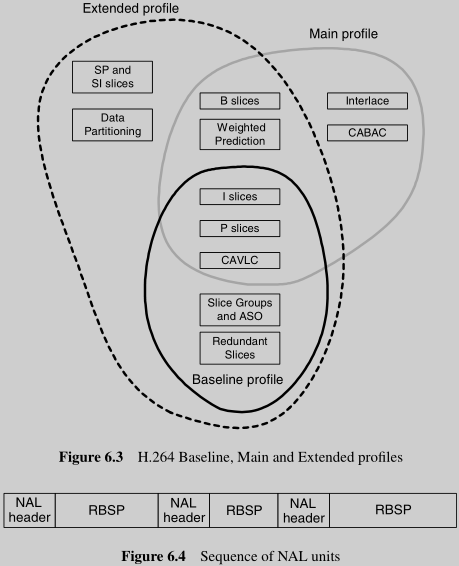
Performance limits for codecs are defined by a set of Levels, each placing limits on parameters such as sample processing rate, picture size, coded bitrate and memory requirements.

RBSP: Raw Byte Sequence Payload

VCL: Video Coding Layer，
NAL: Network Abstraction layer

区分VCL和NAL的原因：VCL层专注coding feature，NAL层专注传输features。

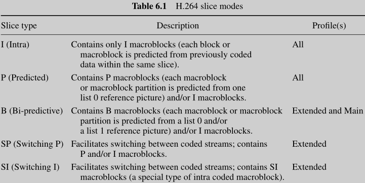
slice最少只有1个macroblock，最多可以包含整个picture的所有marcoblock（1 slice per picture）。一个picture中的所有slice各自包含的macroblock数量不需要相同。slice之间 minimal inter-dependency，这是为了限制error的影响范围。

DPB: Decoded Picture Buffer

IDR：Instantaneous Decoder Refresh，made up of I- or SI- slices， used to clear up the contents of refernece picture buffer. 当decoder收到IDR picture时，decoder marks all pictures in the reference buffer as unused for reference. The first picture is always an IDR picture.

ASO：Arbitrary Slice Order. Slices in a coded picture may follow any decoding order. 只要某个slice的第一个MB的序号，比前面的slice的第一个MB序号要小，就是这个feature了。

slice group，没看懂...

Tree Structured Motion Compensation

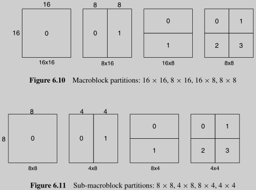
上图的这种划分，全是是针对inter prediction的MB，即只有inter的MB才能够这样做partition。而选择了Intra的MB，划分方式不同，只允许正方形，即为16x161，8x84，或4x416。这是H264的特点。Transform Block的划分是独立的，8x84，或4x4*16。在H.264中，MB是选择prediction scheme的最小单位！

chroma部分等比例缩小操作，包括motion vector。

区块越大，residual的energy就可能越大，但是motion vector数量越小；区块越小，residual的energy就越小，但motion vecotr的数量越大。因此，一般对homogeneous area采用大区块，这样residual的energy也不会很大，对有很多detail的area，采用小区块。

six tap Finite Impulse Response (FIR) filter withweights (1/32, -5/32, 5/8, 5/8, -5/32, 1/32)。这是在做 interpolation 的时候用的方法， interpolation是为了做sub-sample motion compensation，还是 half-pel sample。做quarter-pel sample时，就用 linear interpolation。（此时产生的 motion vector 是 float number）

Motion Vector Prediction

每个partition都需要一个motion vector，这需要很多bits来coding，特别是在partition很小的时候。同时，相邻partition的motion vector具有强相关性，因此就有了用相邻的partition的vector来预测当前partition的vector的条件。跟motion compensation一样，有一个预测是vector，MVp，还有MVD，motion vector difference！

Intra Prediction

4x4 luma block has 9 optional modes, 16x16 has 4 modes, and 4 modes for chroma components.

一种特殊的intra mode，I_PCM，直接传输 image samples，不做prediction，transform，quantization 和 entropy coding。在一些特殊的场景，比如特别异常的 image content，这种模式可能会更有效率。I_PCM模式可以给出一个MB bits数的绝对限制，而不影响画面质量。

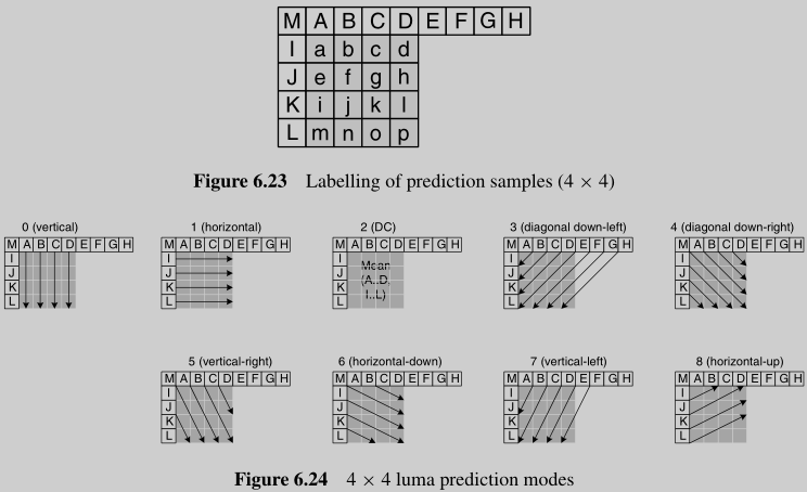
对于 mode 3 -- 8， the predicted samples are formed from a weighted average of prediction samples. （书中没有给出具体的weights）用SAE这个指标来判断和选择效果最好mode！

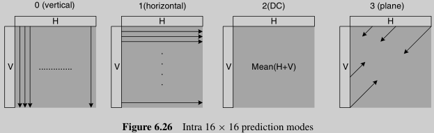
Mode 3 Plane: A linear plane function is fitted to the upper and left-hand samples H and V. This works well in areas of smoothly-varying luminance.

对于8x8 Chroma Prediction Modes，编号不太一样：

mode 0： DC
mode 1： horizontal
mode 2： vertical
mode 3： plane

对于4x4的相邻block的intra mode也是强相关的，老规矩，用predictive coding来signalling intra prediction mode。（16x16的block和chroma block，不使用这个方法）

所谓predictive coding，其实就是通过某种方式来得到一份prediction，prediction和true value之间有个difference（residual），给解码端发送得到prediction的方法以及difference。

Deblocking Filter

A filter is applied to each decoded macroblock to reduce blocking distortion. The deblocking filter is applied just after the inverse transform. The filter smooths block edges, improving the appearance of decoded frames.

When QP is larger, blocking distortion is likely to be more significant.

H.264有3种transform：

Hadamard transform for the 4x4 array of luma DC coefficients in intra MB predicted in 16x16 mode,
Hadamard transform for the 2x2 array of chroma DC coefficients,
a DCT-based transform for all other 4x4 blocks in residual data.

transformed data 的传输顺序：

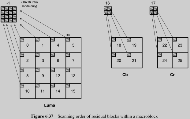
从 -1 到 25 这个顺序。

H.264的transform基于DCT，但是也有很大的不同！

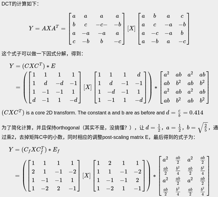
为什么要这样计算？

transform计算过程全是integer（16 bits），在decoding的时候，没有精度损失，zero mismatch；
transform的核心计算，可以只有加法和移位；
最后处理E矩阵，这一步操作并入quantization，减少做乘法的次数；

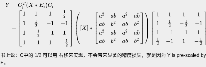
inverse transform的计算公式：

DCT矩阵是正交的，DCT和IDCT是可逆的：

>>> a
array([[ 0.5  ,  0.5  ,  0.5  ,  0.5  ],
       [ 0.653,  0.271, -0.271, -0.653],
       [ 0.5  , -0.5  , -0.5  ,  0.5  ],
       [ 0.271, -0.653,  0.653, -0.271]])
>>> np.round(a @ a.T)
array([[ 1.,  0.,  0.,  0.],
       [ 0.,  1.,  0., -0.],
       [ 0.,  0.,  1.,  0.],
       [ 0., -0.,  0.,  1.]])
>>> x
array([[ 5, 11,  8, 10],
       [ 9,  8,  4, 12],
       [ 1, 10, 11,  4],
       [19,  6, 15,  7]])
>>> y = a @ x @ a.T
>>> y
array([[35.      , -0.08    , -1.5     ,  1.115   ],
       [-3.296   , -4.758192,  0.449   , -9.010094],
       [ 5.5     ,  3.025   ,  2.      ,  4.7     ],
       [-4.047   , -3.011894, -9.382   , -1.240008]])
>>> x2 = a.T @ y @ a
>>> x2
array([[ 5.00284962, 10.99880027,  8.00149973,  9.99880038],
       [ 8.99925   ,  7.99970011,  4.00164989, 11.99835   ],
       [ 1.00165   ,  9.99984989, 10.99880011,  4.00075   ],
       [18.99610038,  6.00209973, 14.99760027,  7.00224962]])
>>> np.round(x2)
array([[ 5., 11.,  8., 10.],
       [ 9.,  8.,  4., 12.],
       [ 1., 10., 11.,  4.],
       [19.,  6., 15.,  7.]])

Nice.....

在H.264之前，video coding标准没有规定具体的IDCT算法，只是要求了一个精度统计测试，这带来了可能 drift（mismatch between the decoded data in the encoder and decoder）。消除 drift 的方法就是要统一算法。DCT的计算有无理数，浮点数，有精度上的问题，同时浮点数计算对某些硬件会带来复杂性，因此H.264开始，提出了 integer transforms，用整数的加减和位移，来代替浮点数计算，降低复杂度。（论文：Low Complexity Transform and Quantization in H.264/AVC）

量化时：（1）避免浮点数出发，这应该是考虑到硬件的成本；（2）包含上文描述的scaling。H264一共有52个Qstep value，QP是这52个值的index。QP ofr Chroma is derived from QP of luma, 也可以自定义QPy和QPc之间的mapping，在PPS包中传递这些信息。

如前所述，如果MB是intra的预测模式，还要对4x4的DC coefficients再次进行hadamard transform。不详细记录了，还有chroma部分的transform，需要的时候再仔细研究。

H.264的prediction和transform的关系：当inter时，如果有小于8x8的partition，要用4x4的transform；当intra时，8x84和4x416，这两种划分，prediction和transform相同，只有在16x161时，先做4x416的transform，然后对DC values再做一次4x4的Hadamard Transform。这样的关系，在代码编写时，会稍显复杂。

下面是MAIN PROFILE的一些记录，前面是内容属于BASELINE。

B slices，reference picture可以一个来自past，一个来自future，也可以两个都来自past，或两个都来自future。B slices使用 list0和list1，这两个list含有short term和long term，这两个list也都可以含有past和future。

Prediction Options:

Direct: skipped MB in B slices
List0
List1
Bi-prediction: 分别从list0和list1中得到两个参考区域，对这两个区域取平均：pred(i,j)=(pred0(i,j)+pred1(i,j)+1)>>1

weighted prediction

echo prediction sample pred0(i,j) or pred1(i,j) is scaled by a weighting factor w0 or w1 prior to motion-compensated prediction. In the explicit types, the weighting factors are determined by the encoder and transmitted in the slice header. If implicit prediction is used, w0 and w1 are calculated based on the relative temporal position of the list0 and list1 reference picture. 这个距离越近，w越大。应用场景：fade transition where one scene fades into another.

EXTENDED PROFILE，很适合video stream，stream的特点是switching，在不同的stream之间切换（内容不同，或者内容相同但bitrate不同）。

一种switching的方案是有规律的插入I-slice（假设frame就一个slice），这些插入点就是switching point，I-slice的decode不需要reference。这种方案有个问题，在switching point，bitrate会出现peak，因为I-slice体量较大。

SP-slice用来在相同内容的不同bitrate的stream中切换使用：

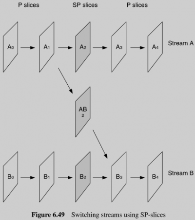
AB2的关键，参考A1，生成B2，有了B2，就可以继续decode B3.......

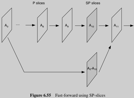
SP-slice的另一个作用是提供fast forward的功能，

还有个相似的SI-slice，书中介绍很少。

[B frame]

B picture or B frame (bipredictive coded picture) – contains motion-compensated difference information relative to previously decoded pictures. In older designs such as MPEG-1 and H.262/MPEG-2, each B picture can only reference two pictures, the one which precedes the B picture in display order and the one which follows, and all referenced pictures must be I or P pictures. These constraints do not apply in newer standards H.264/MPEG-4 AVC and HEVC.

[P frame]

P picture or P frame (predictive coded picture) – contains motion-compensated difference information relative to previously decoded pictures. In older designs such as MPEG-1, H.262/MPEG-2 and H.263, each P picture can only reference one picture, and that picture must precede the P picture in display order as well as in decoding order and must be an I or P picture. These constraints do not apply in the newer standards H.264/MPEG-4 AVC and HEVC.

关于P和B slice：P Slice里所有帧间预测的预测块只能有一个运动补偿预测信息。P Slice只能有一个参考图像列表。B Slice里所有帧间预测的预测块最多可以有两个运动补偿预测信息，B Slice可以使用两个参考图像列表。reference picture list里面可以存放多张图片哦。

P-frames provide the “differences” between the current frame and one (or more) frames that came before it. P-frames offer much better compression than I-frames, because they take advantage of both temporal and spatial compression and use less bits within a video stream.

H.264/AVC uses a 6-tap filter for half-pixel interpolation and then simple linear interpolation to achieve quarter-pixel precision from the half-pixel data. 从书中的说明来分析，决定如何划分一个MB，还是要分析residual data，变化不大，partition就大，变化不小，partition就小。

The terms sub-pixel, half-pixel and quarter-pixel are widely used in this context although in fact the processis usually applied to luma and chroma samples, not pixels.

本文链接：https://cs.pynote.net/ag/image/202211052/

-- EOF --

-- MORE --