Last Updated: 2024-03-20 08:32:55 Wednesday
-- TOC --
大规模数组或矩阵计算,在Python生态中,只有NumPy!《nature》上的一篇文章:Array programming with NumPy
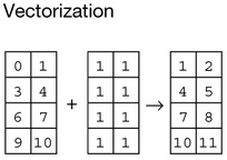
Vectorization, operating on entire arrays rather than their individual elements, is essential toarray programming. This means that operations that would take many tens of lines to express in languages such as C can often be implemented as a single, clear Python expression.
从形式上看,vectorization就是没有循环(循环在看不见的底层进行)!有循环就慢了...而且需要写的代码更多,更容易出错。vectorization语句的表达力很强悍!
NumPy官网:https://numpy.org/
Python is an open-source, general-purpose interpreted programming language well suited to standard programming tasks such as cleaning data, interacting with web resources and parsing text. Adding
fast array operations and linear algebraenables scientists to do all their work within a single programming language, one that has the advantage of being famously easy to learn and teach, as witnessed by its adoption as a primary learning language in many universities.
Import NumPy to Python code:
import numpy as np
本文的示例代码,全都使用np这个非常通用的name。
有一些图像计算方面的操作,使用openCV比NumPy更快,比如cv2.cvtColor接口将BGRA数据转RGB。
ndarray,a homogeneous n-dimensional array object, with methods to efficiently operate on it. 它是NumPy用来表达各种shape和dtype的array的对象,matrix或tensor这样的概念,都可用不同参数的ndarray对象表达。
ndarray.ndim,the number of axes (dimensions) of the array,维度。
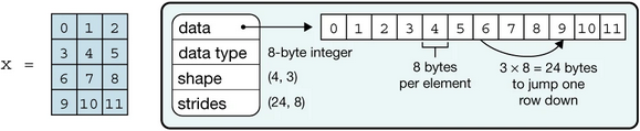
ndarray.shape,the dimensions of the array. This is a tuple of integers indicating the size of the array in each dimension. For a matrix with n rows and m columns, shape will be (n,m). The length of the shape tuple is therefore the number of axes, ndim。形态。
ndarray.size,the total number of elements of the array. This is equal to the product of the elements of shape,元素的数量。
ndarray.dtype,an object describing the type of the elements in the array,元素的类型。
如果把ndarray看作container,其要求所有element必须具有相同dtype!
ndarray.itemsize,the size in bytes of each element of the array. For example, an array of elements of type float64 has itemsize 8 (=64/8), while one of type complex32 has itemsize 4 (=32/8). It is equivalent to ndarray.dtype.itemsize。元素的大小,byte size。
ndarray.data,the buffer containing the actual elements of the array. Normally, we won’t need to use this attribute because we will access the elements in an array using indexing facilities。数据区。
ndarray.strides,are necessary to interpret computer memory, which stores elements linearly, as multidimensional arrays. They describe the number of bytes to move forward in memory to jump from row to row, column to column, and so forth. Consider, for example, a two-dimensional array of floating-point numbers with shape (4,3), where each element occupies 8 bytes in memory. To move between consecutive columns, we need to jump forward 8 bytes in memory, and to access the next row, jump 3 × 8 = 24 bytes. The strides of that array are therefore (24,8). NumPy can store arrays in either C or Fortran memory order, iterating first over either rows or columns. This allows external libraries written in those languages to access NumPy array data in memory directly.
NumPy使用axis这个词来代表维度,axis的复数是axes,我们一般说,一个ndarray有多少axis,就是表示它有几个维度。真正的数据本身,都是在最高维度内存放着的!低维度的axis,逻辑上表达的只是其它axis而已。
ndaraay.flags,属性,比如read-only等,
>>> help(np.ndarray.flags)
用np.frombuffer得到的ndarray有read-only属性。
下面以代码示例的形式,介绍围绕ndarray对象的常用操作接口。
np.array
将list或tuple直接转ndarray对象:
>>> a = [i for i in range(100)]
>>> aa = np.array(a)
>>> aa
array([ 0,  1,  2,  3,  4,  5,  6,  7,  8,  9, 10, 11, 12, 13, 14, 15, 16,
       17, 18, 19, 20, 21, 22, 23, 24, 25, 26, 27, 28, 29, 30, 31, 32, 33,
       34, 35, 36, 37, 38, 39, 40, 41, 42, 43, 44, 45, 46, 47, 48, 49, 50,
       51, 52, 53, 54, 55, 56, 57, 58, 59, 60, 61, 62, 63, 64, 65, 66, 67,
       68, 69, 70, 71, 72, 73, 74, 75, 76, 77, 78, 79, 80, 81, 82, 83, 84,
       85, 86, 87, 88, 89, 90, 91, 92, 93, 94, 95, 96, 97, 98, 99])
>>> aa.shape
(100,)  # different with (100,1) which is 2 dimensions
>>> aa.ndim
1
>>> aa.dtype
dtype('int64')
>>> aa.size
100
>>> aa.itemsize
8
>>> aa.strides
(8,)
>>> aa.data
<memory at 0x7feddf177d00>
嵌套list直接转多维array:
>>> b = [[i*j for i in range(4)] for j in range(5)]
>>> ba = np.array(b)
>>> ba.shape
(5, 4)
>>> ba
array([[ 0,  0,  0,  0],
       [ 0,  1,  2,  3],
       [ 0,  2,  4,  6],
       [ 0,  3,  6,  9],
       [ 0,  4,  8, 12]])
如果list或tuple中的数据类型不一致,在转ndarray对象时,存在转换:
>>> c = (1,2,3,4,5.0)  # 5.0 is the last element
>>> ca = np.array(c)
>>> ca.dtype
dtype('float64')
创建array时指定dtype:
>>> d = (1,2,3,4,5.0)
>>> da = np.array(d, dtype=np.int32)
>>> da
array([1, 2, 3, 4, 5], dtype=int32)
np.matrix
与np.array很相似。
np.asarray
将输入转换为ndarray,跟np.array比较相似。
np.zeros
用指定的shape和dtype创建全0的ndarray对象:
>>> za = np.zeros((3,4), dtype=np.float32)
>>> za
array([[0., 0., 0., 0.],
       [0., 0., 0., 0.],
       [0., 0., 0., 0.]], dtype=float32)
np.zeros_like
按照某个ndarray对象的shape,以及指定的dtype,创建新的ndarray对象:
>>> t = [[[i+j+k for i in range(3)] for j in range(4)] for k in range(5)]
>>> ta = np.array(t)
>>> zta = np.zeros_like(ta, dtype=np.float16)
>>> zta
array([[[0., 0., 0.],
        [0., 0., 0.],
        [0., 0., 0.],
        [0., 0., 0.]],

       [[0., 0., 0.],
        [0., 0., 0.],
        [0., 0., 0.],
        [0., 0., 0.]],

       [[0., 0., 0.],
        [0., 0., 0.],
        [0., 0., 0.],
        [0., 0., 0.]],

       [[0., 0., 0.],
        [0., 0., 0.],
        [0., 0., 0.],
        [0., 0., 0.]],

       [[0., 0., 0.],
        [0., 0., 0.],
        [0., 0., 0.],
        [0., 0., 0.]]], dtype=float16)
>>> zta.shape
(5, 4, 3)
np.ones
跟np.zeros函数一样,创建全1的ndarray对象。
np.ones_like
跟np.zeros_like函数一样,全1而已。
np.empty
跟np.zeros和np.ones一样,而不一样的地方在于,np.empty接口不对数据做初始化,即所有的内部数据都是随机的,使用np.empty接口,可以进一步提高计算速度。
>>> ea = np.empty((2,2), dtype=np.int32)
>>> ea
array([[          0, -1073741824],
       [ -558661633,       32749]], dtype=int32)
np.empty_like
跟其它*_like接口一样,也跟np.empty一样,不做初始化。
np.arange
用类似range的方式(Python内置的range接口)创建ndarray,只是start/stop/step都可以使用float类型的数据:
>>> ra = np.arange(10)  # default dtype is int
>>> ra
array([0, 1, 2, 3, 4, 5, 6, 7, 8, 9])
>>> ra.shape
(10,)
>>> ra.dtype
dtype('int64')
>>>
>>> ra = np.arange(0,10,3)
>>> ra
array([0, 3, 6, 9])
>>>
>>> ra = np.arange(0, 1, 0.1)  # float step
>>> ra
array([0. , 0.1, 0.2, 0.3, 0.4, 0.5, 0.6, 0.7, 0.8, 0.9])
>>> ra.dtype
dtype('float64')
>>>
>>> ra = np.arange(0.1, 0.2, 0.01)  # float start and stop
>>> ra
array([0.1 , 0.11, 0.12, 0.13, 0.14, 0.15, 0.16, 0.17, 0.18, 0.19])
np.arange接口有个坑需要注意:
>>> ra = np.arange(1, 5, 0.8, dtype=np.int32)
>>> ra
array([1, 1, 1, 1, 1], dtype=int32)
为什么是全1?很可能是np.arange接口内部在迭代的时候,每生成一个数,就做一次类型转换(C风格的强转),然后在结果的基础上step得到下一个数,然后再转换,这样就得到的全是1。要避免这样的坑,使用下面的np.linspace接口。
np.linspace
设置start和stop,设置均匀分割数量n,inclusive,可指定数据类型:
>>> la = np.linspace(1,4,7)
>>> la
array([1. , 1.5, 2. , 2.5, 3. , 3.5, 4. ])
>>> la = np.linspace(1,4,7, dtype=np.int32)
>>> la
array([1, 1, 2, 2, 3, 3, 4], dtype=int32)
np.linspace接口有个参数endpoint,默认为True。
np.reshape
将一个ndarray的shape进行变换,变换之后,维度可能发生变化:
>>> a = np.array((1,2,3,4,5,6)).reshape(2,3)
>>> a.shape
(2, 3)
>>> b = np.arange(100).reshape(4,5,5)
>>> b.shape
(4, 5, 5)
>>> c = np.linspace(1,100,1000).reshape(10,10,10)
>>> c.shape
(10, 10, 10)
以上代码都是在ndarray对象上调用reshape接口,我们也可以直接调用np.reshape接口,并且使用-1来进行自动计算:
>>> a.shape
(4, 6)
>>> np.reshape(a,(3,-1)).shape
(3, 8)
>>> np.reshape(a,(-1,4)).shape
(6, 4)
np.eye
创建单位矩阵Identity matrix:
>>> I = np.eye(3, dtype=np.int8)
>>> I
array([[1, 0, 0],
       [0, 1, 0],
       [0, 0, 1]], dtype=int8)
np.full
用同一个固定的数字来填满ndarray中所有空间:
zeros是用0填,ones是用1填,empty不填。
>>> d = np.full((2,3,4),9,dtype=np.uint8)
>>> d
array([[[9, 9, 9, 9],
        [9, 9, 9, 9],
        [9, 9, 9, 9]],

       [[9, 9, 9, 9],
        [9, 9, 9, 9],
        [9, 9, 9, 9]]], dtype=uint8)
Array-aware functionrefers to the function that can operate on NumPy arrays in anelement-wise manner. This means that the function can take an array as input and perform its operation on each individual element of the array, without having to manually loop through each element.
NumPy提供了很多array-aware function:
np.sin
np.cos
np.tan
np.exp
np.log
np.sqrt
np.power
np.absolute
np.round
np.floor
...
Broadcasting is a way of applying operations between two arrays with different shapes. When you perform an operation between two arrays, NumPy will automatically try to align their shapes so that they can be operated on together.
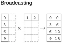
比如scalar和array的运算(broadcast也有element-wise的效果):
>>> a = np.array((1,2,3,4))
>>> a + 1
array([2, 3, 4, 5])
>>> a - 1
array([0, 1, 2, 3])
>>> a * 2
array([2, 4, 6, 8])
>>> a / 2
array([0.5, 1. , 1.5, 2. ])
>>> a**2  # np.power(a, 2)
array([ 1,  4,  9, 16])
比如不同shape的ndarray之间的运算:
>>> a
array([[0, 1],
       [2, 3]])
>>> b  # b is just like to be expanded with a new row [1,2]!
array([[1, 2]])
>>> a + b
array([[1, 3],
       [3, 5]])
>>> a - b
array([[-1, -1],
       [ 1,  1]])
>>> a * b
array([[0, 2],
       [2, 6]])
>>> a / b
array([[0. , 0.5],
       [2. , 1.5]])
>>> a**b
array([[0, 1],
       [2, 9]])
比较操作也一样broadcasting:
>>> a < b
array([[ True,  True],
       [False, False]])
如果两个ndarray对象shape一样,就不需要broadcasting了,直接element-wise进行计算。不管是否broadcasting,都体现了NumPy的Vectorization的特性!不需要把broadcasting像的太复杂,其实它就是一种将不同shape的ndarray的shape变成一样的机制。
*,表示elementwise的乘法,这种乘法叫Hadamard Product。@或者np.dot接口,就是标准的矩阵乘法。np.prod接口与np.sum接口类似。>>> a = np.arange(25).reshape(5,5)
>>> a
array([[ 0, 1, 2, 3, 4],
[ 5, 6, 7, 8, 9],
[10, 11, 12, 13, 14],
[15, 16, 17, 18, 19],
[20, 21, 22, 23, 24]])
>>> a * a # Hadamard Product
array([[ 0, 1, 4, 9, 16],
[ 25, 36, 49, 64, 81],
[100, 121, 144, 169, 196],
[225, 256, 289, 324, 361],
[400, 441, 484, 529, 576]])
>>> a @ a # Matrix Product
array([[ 150, 160, 170, 180, 190],
[ 400, 435, 470, 505, 540],
[ 650, 710, 770, 830, 890],
[ 900, 985, 1070, 1155, 1240],
[1150, 1260, 1370, 1480, 1590]])
>>> np.dot(a,a) # same with @
array([[ 150, 160, 170, 180, 190],
[ 400, 435, 470, 505, 540],
[ 650, 710, 770, 830, 890],
[ 900, 985, 1070, 1155, 1240],
[1150, 1260, 1370, 1480, 1590]])
np.prod
这个接口与np.sum类似,后者计算和,前者计算乘积。
当计算结果是一个ndarray对象时,默认是创建一个新的ndarray。而如果表达式使用类似于 += or *= 这样的Augmented Assignment Operator,就不会创建新的ndarray,就地修改原来的。
>>> a
array([[ 0,  1,  2,  3,  4],
       [ 5,  6,  7,  8,  9],
       [10, 11, 12, 13, 14],
       [15, 16, 17, 18, 19],
       [20, 21, 22, 23, 24]])
>>> id(a)
3039556576
>>> a = a + 1  # a is a new ndarray
>>> id(a)
3039556776
>>> a += 1     # in-place modification
>>> id(a)
3039556776
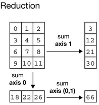
np模块提供的很多函数接口,比如np.sum,都有axis参数,这个参数的含义是,沿着指定的axis进行计算!
>>> a = np.arange(6).reshape(2,3)
>>> a
array([[0, 1, 2],
       [3, 4, 5]])
>>> np.sum(a, axis=0)  # summing along row
array([3, 5, 7])
>>> np.sum(a, axis=1)  # summing along column
array([ 3, 12])
按axis计算后,一般都伴随着降低维度的效果。比如2维数组,无论是沿着row或column计算sum,结果都是1维数组。
>>> a = np.arange(24).reshape(2,3,4)
>>> a
array([[[ 0,  1,  2,  3],
        [ 4,  5,  6,  7],
        [ 8,  9, 10, 11]],

       [[12, 13, 14, 15],
        [16, 17, 18, 19],
        [20, 21, 22, 23]]])
>>> np.sum(a, axis=0)
array([[12, 14, 16, 18],
       [20, 22, 24, 26],
       [28, 30, 32, 34]])
>>> np.sum(a, axis=1)
array([[12, 15, 18, 21],
       [48, 51, 54, 57]])
>>> np.sum(a, axis=2)
array([[ 6, 22, 38],
       [54, 70, 86]])
>>> a = np.array([1,2,3,4,5,6,7,8,9])
>>> np.mean(a)
5.0
np.mean函数有axis参数可以使用:
>>> a
array([[ 0,  1,  2,  3,  4],
       [ 5,  6,  7,  8,  9],
       [10, 11, 12, 13, 14],
       [15, 16, 17, 18, 19]])
>>> a.shape
(4, 5)
>>> np.mean(a, axis=0)
array([ 7.5,  8.5,  9.5, 10.5, 11.5])
>>> np.mean(a, axis=1)
array([ 2.,  7., 12., 17.])
>>> np.mean(a, axis=(0,1))
9.5
>>> np.mean(a)
9.5
除了np.mean函数,还有np.average函数也可以用来计算均值,不一样的地方是,np.average函数可以带一个weights参数。
reduction后,维度会减少,NumPy中很多接口,都有keepdims参数,如果keepdims=True,维度得到保持,不会减少。
默认ndarray的打印输出已经很完美了,但对于size很大的ndarray,打印时会自动进行裁剪,如果不想裁剪,要么自己写loop,或者:
>>> np.set_printoptions(threshold=sys.maxsize)
显然,用多重循环来遍历ndarray,效率是非常低的。
np.flat
得到一个iterator:
>>> a = np.arange(4).reshape(2,2)
>>> for i in a.flat:
...   print(i)
...
0
1
2
3
np.ravel
得到一个新的一维ndarray:
>>> a = np.arange(120).reshape(2,3,4,5)
>>> b = a.ravel()
>>> b.shape
(120,)
The order of the elements in the array resulting from ravel() is normally
C-style, that is, the rightmost index “changes the fastest”, so the elementafter a[0,0] is a[0,1]. If the array is reshaped to some other shape, again the array is treated as “C-style”.
np.reshape
改变shape,得到一个新的ndarray,前文已介绍。
np.resize
与np.reshape不同的是,np.resize就地变形,不会生产新的ndarray对象。
>>> a.shape
(5, 20)
>>> id(a)
3040477536
>>> a.resize(20,5)
>>> a.shape
(20, 5)
>>> id(a)
3040477536
T / np.transpose
转置会生成新的矩阵,使用T或np.transpose接口:
>>> a = np.arange(6).reshape(2,3)
>>> a.shape
(2, 3)
>>> a.T.shape
(3, 2)
>>> np.transpose(a).shape
(3, 2)
np.ravel
生成一维的ndarray,前文已介绍。
np.newaxis
增加ndarray的维度:
>>> a = np.array((1,2,3,4))
>>> a.shape
(4,)
>>> a[np.newaxis,:].reshape(2,2).shape
(2, 2)
>>> a[np.newaxis,:,np.newaxis].shape
(1, 4, 1)
np.expand_dims
用来增加ndarray的维度,用法如下:
>>> a = np.arange(10).reshape(2,5)
>>> a.shape
(2, 5)
>>> np.expand_dims(a, axis=0).shape
(1, 2, 5)
>>> np.expand_dims(a, axis=1).shape
(2, 1, 5)
>>> np.expand_dims(a, axis=2).shape
(2, 5, 1)
astype用来转换dtype,但需要注意这种转换可能带来的问题,比如数据精度丢失,数据异常:
>>> a
>>> a = np.array((-2,-1,0,1,2))
>>> a
array([-2, -1,  0,  1,  2])
>>> b = a.astype(np.uint8)
>>> b
array([254, 255,   0,   1,   2], dtype=uint8)
前文已经介绍转置可用用T属性或np.transpose接口。这里补充非二维ndarray,也一样可以转置:
>>> a.shape
(2, 3, 4, 5)
>>> a.T.shape
(5, 4, 3, 2)
>>> np.transpose(a).shape
(5, 4, 3, 2)
还可以通过指定axis的方式,进行任意转置:
>>> a.shape
(2, 3, 4, 5)
>>> np.transpose(a, (0,2,1,3)).shape
(2, 4, 3, 5)
>>> np.transpose(a, (3,2,1,0)).shape
(5, 4, 3, 2)
>>> np.transpose(a, (3,0,1,2)).shape
(5, 2, 3, 4)
维度为1的array,就是个普通数组,我的经验是,1维ndarray在计算时会被当作行向量处理,比如broadcasting,扩展的是row。而列向量是2维的,只是有个维度是1而已。
>>> array = np.array((1,2,3,4,5))
>>> array
array([1, 2, 3, 4, 5])  # only one pair of []
>>> array.shape
(5,)                    # dimension is 1
>>> vector = array.reshape(5,1)
>>> vector
array([[1],             # nested []
       [2],
       [3],
       [4],
       [5]])
>>> vector.shape
(5, 1)                 # dimension is 2
1维ndarray的broadcasting:
>>> a
array([1, 2, 3, 4])
>>> b
array([[ 0,  1,  2,  3],
       [ 4,  5,  6,  7],
       [ 8,  9, 10, 11]])
>>> b + a
array([[ 1,  3,  5,  7],
       [ 5,  7,  9, 11],
       [ 9, 11, 13, 15]])
选出满足条件的所有元素
>>> a = np.arange(24).reshape(2,3,4)  # ndim = 3
>>> a[a<12]                           # ndim = 1
array([ 0,  1,  2,  3,  4,  5,  6,  7,  8,  9, 10, 11])
修改满足条件的元素
>>> a[a<12] = 12  # a = np.where(a<12, 12, a)
>>> a
array([[[12, 12, 12, 12],
        [12, 12, 12, 12],
        [12, 12, 12, 12]],

       [[12, 13, 14, 15],
        [16, 17, 18, 19],
        [20, 21, 22, 23]]])
布尔矩阵
如果用ndarray直接做条件判断,会得到一个全是True和False的shape一样的ndarray:
>>> a
array([[0, 1, 2, 3, 4],
       [5, 6, 7, 8, 9]])
>>> a > 3
array([[False, False, False, False,  True],
       [ True,  True,  True,  True,  True]])
>>> a > 5
array([[False, False, False, False, False],
       [False,  True,  True,  True,  True]])
常常看到配合使用np.sum的代码,用来统计满足条件的元素个数:
>>> np.sum(a>3)
6
>>> np.sum(a>5)
4
将布尔矩阵转换为01矩阵
有的时候,我们需要将全为True和False的矩阵,转换成全为0或1:
>>> b = (a>5).astype(np.uint8)
>>> b
array([[0, 0, 0, 0, 0],
       [0, 1, 1, 1, 1]], dtype=uint8)
用np.nonzero精确定位
如果再配合上np.nonzero函数,就可以把符合我们条件的数据的位置找出来。比如这个找出所有大于6的数据的位置:
>>> a
array([[0, 1, 2, 3, 4],
       [5, 6, 7, 8, 9]])
>>> b = (a>6)
>>> b
array([[False, False, False, False, False],
       [False, False,  True,  True,  True]])
>>> c = np.nonzero(b)
>>> c
(array([1, 1, 1], dtype=int64), array([2, 3, 4], dtype=int64))
>>>
>>> b[c[0],c[1]]
array([ True,  True,  True])
>>> b[np.nonzero(b)]
array([ True,  True,  True])
>>>
>>> a[c[0],c[1]]
array([7, 8, 9])
>>> a[np.nonzero(b)]
array([7, 8, 9])
c是tuple,c[0]指定row,c[1]指定column。后面有对这种选择元素方法的专门介绍。
下面再试一个3D的ndarray,找出所有大于6并小于16的数据位置:
>>> a = np.arange(24).reshape(2,3,4)
>>> a
array([[[ 0,  1,  2,  3],
        [ 4,  5,  6,  7],
        [ 8,  9, 10, 11]],

       [[12, 13, 14, 15],
        [16, 17, 18, 19],
        [20, 21, 22, 23]]])
>>> a.shape
(2, 3, 4)
>>> b = (a>6)&(a<16)  # two matrix do AND
>>> b
array([[[False, False, False, False],
        [False, False, False,  True],
        [ True,  True,  True,  True]],

       [[ True,  True,  True,  True],
        [False, False, False, False],
        [False, False, False, False]]])
>>> c = np.nonzero(b)
>>> c
(array([0, 0, 0, 0, 0, 1, 1, 1, 1], dtype=int64), array([1, 2, 2, 2, 2, 0, 0, 0,
 0], dtype=int64), array([3, 0, 1, 2, 3, 0, 1, 2, 3], dtype=int64))
>>> b[c[0],c[1],c[2]]
array([ True,  True,  True,  True,  True,  True,  True,  True,  True])
>>> a[c[0],c[1],c[2]]
array([ 7,  8,  9, 10, 11, 12, 13, 14, 15])
np.flatnonzero
将输入的ndarray作flat,返回nonzero的index。
np.where
np.where可以直接修改满足条件的元素的值:
>>> b
array([[1, 2, 3],
       [2, 3, 4],
       [1, 1, 1]])
>>> b = np.where(b==1,0,b)
>>> b
array([[0, 2, 3],
       [2, 3, 4],
       [0, 0, 0]])
将满足条件的元素赋值为0,其它不变。
>>> b = np.where(b==0,-1,5)
>>> b
array([[-1,  5,  5],
       [ 5,  5,  5],
       [-1, -1, -1]])
将满足条件的元素赋值为-1,其它赋值为5。
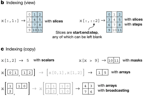
首先,一般我们的index都是tuple:
>>> a.shape
(4, 5, 5)
>>> a[0,2,4]  # no ()
14
>>> a[(0,2,4)]
14
当使用List作为Index的时候,含义发生了变化:
>>> a[[0,2]]
array([[[ 0,  1,  2,  3,  4],
        [ 5,  6,  7,  8,  9],
        [10, 11, 12, 13, 14],
        [15, 16, 17, 18, 19],
        [20, 21, 22, 23, 24]],

       [[50, 51, 52, 53, 54],
        [55, 56, 57, 58, 59],
        [60, 61, 62, 63, 64],
        [65, 66, 67, 68, 69],
        [70, 71, 72, 73, 74]]])
将List中数字所代表的维度整体取出来,组成一个新的ndarray对象。这种操作,可以在多个维度执行:
>>> a[[0,2],[1,3]]
array([[ 5,  6,  7,  8,  9],
       [65, 66, 67, 68, 69]])
>>> a[0,1,:]
array([5, 6, 7, 8, 9])
>>> a[2,3,:]
array([65, 66, 67, 68, 69])
>>> a[(0,2),(1,3)]
array([[ 5,  6,  7,  8,  9],
       [65, 66, 67, 68, 69]])
此时使用tuple,与使用list,就成了一样的了!使用ndarray对象,也是OK的。
这种方式不仅仅可以用来选出符合复杂条件的元素,还可以直接对这些符合条件的位值进行赋值操作:
>>> a = np.arange(24).reshape(2,3,4)
>>> a
array([[[ 0,  1,  2,  3],
        [ 4,  5,  6,  7],
        [ 8,  9, 10, 11]],

       [[12, 13, 14, 15],
        [16, 17, 18, 19],
        [20, 21, 22, 23]]])
>>> a[(0,1),(1,2),(2,3)]
array([ 6, 23])
>>> a[(0,1),(1,2),(2,3)] = -1  # !!
>>> a
array([[[ 0,  1,  2,  3],
        [ 4,  5, -1,  7],
        [ 8,  9, 10, 11]],

       [[12, 13, 14, 15],
        [16, 17, 18, 19],
        [20, 21, 22, -1]]])
BGRA数据转RGB
# height 926, width 1614, BGRA
>>> img = np.frombuffer(bgra_data, dtype=np.uint8).reshape(926,1614,4)
>>> img_rgb = img[:,:,(2,1,0)]
实际上,BGRA转RGB这个动作,用openCV接口更快!
ndarray对象可以转换为Python内置的list对象。
>>> a = np.array((1,2,3,4))
>>> a.tolist()
[1, 2, 3, 4]
>>> list(a)
[1, 2, 3, 4]
对于多维ndarray对象,在转list时,接口的功能是不同的:
>>> a = np.arange(8).reshape(4,2)
>>> a.tolist()
[[0, 1], [2, 3], [4, 5], [6, 7]]
>>> list(a)
[array([0, 1]), array([2, 3]), array([4, 5]), array([6, 7])]
这里补充前述内容没有覆盖到的NumPy接口。
这是两个常用接口,用来得到各个维度的最大或最小index。
>>> a = np.random.randn(3,4)
>>> a
array([[ 0.30346114, -2.29243679,  0.52973608,  0.04204178],
       [ 0.80209999,  0.58868945,  0.99432318,  1.64219216],
       [-0.0914746 , -0.12801855,  0.09728936,  0.40889348]])
>>> np.argmax(a, axis=0)
array([1, 1, 1, 1])
>>> np.argmax(a, axis=1)
array([2, 3, 3])
>>> np.argmin(a, axis=0)
array([2, 0, 2, 0])
>>> np.argmin(a, axis=1)
array([1, 1, 1])
按各维度进行排序,得到一组indexes。
>>> a
array([[41, 32, 57, 71, 23, 35],
       [56,  2, 52, 17, 36, 79],
       [73, 18,  1, 80,  7, 65],
       [82, 76, 36, 89, 28, 11]])
>>> np.argsort(a)
array([[4, 1, 5, 0, 2, 3],
       [1, 3, 4, 2, 0, 5],
       [2, 4, 1, 5, 0, 3],
       [5, 4, 2, 1, 0, 3]])
有
arg的都是得到indexes。
找出最大值或最小值,可以设置axis参数。
对两个ndarray(broadcasting)进行element-wise的大小取舍,生成一个新的ndarray:
>>> a
array([[0, 1, 2, 3, 4],
       [5, 6, 7, 8, 9]])
>>> np.maximum(5, a)
array([[5, 5, 5, 5, 5],
       [5, 6, 7, 8, 9]])
>>> np.minimum(5, a)
array([[0, 1, 2, 3, 4],
       [5, 5, 5, 5, 5]])
>>> a
array([[1, 7, 3, 2, 1, 0],
       [5, 0, 3, 7, 3, 2],
       [6, 4, 0, 7, 6, 0],
       [2, 6, 4, 4, 6, 1]])
>>> np.sort(a)                # sort along the last axis
array([[0, 1, 1, 2, 3, 7],
       [0, 2, 3, 3, 5, 7],
       [0, 0, 4, 6, 6, 7],
       [1, 2, 4, 4, 6, 6]])
>>> np.sort(a,axis=None)      # sort the flattened array
array([0, 0, 0, 0, 1, 1, 1, 2, 2, 2, 3, 3, 3, 4, 4, 4, 5, 6, 6, 6, 6, 7,
       7, 7])
>>> np.sort(a,axis=0)         # sort along the first axis
array([[1, 0, 0, 2, 1, 0],
       [2, 4, 3, 4, 3, 0],
       [5, 6, 3, 7, 6, 1],
       [6, 7, 4, 7, 6, 2]])
判断是否全true或任意true。
>>> a = np.arange(10).reshape(2,5)
>>> np.all(a)
False
>>> np.any(a)
True
>>> np.all(a,axis=0)
array([False,  True,  True,  True,  True])
>>> np.any(a,axis=1)
array([ True,  True])
判断两个ndarray是否相同
这个判断适合非float数据类型的ndarray:
>>> (a==a).all()
True
>>> (a!=a).any()
False
将一段buffer转换为一维的read-only ndarray!
>>> a = np.frombuffer(b'\x00\x01\x02\x03',dtype=np.uint8, count=2, offset=1)  # handy count and offset parameters
array([1, 2], dtype=uint8)
>>> a.flags
  C_CONTIGUOUS : True
  F_CONTIGUOUS : True
  OWNDATA : False
  WRITEABLE : False  # <--- !!!
  ALIGNED : True
  WRITEBACKIFCOPY : False
>>> a.flags.writeable  # can be modified directly
False
np.frombuffer可能存在的byteorder问题处理
>>> dt = np.dtype(np.uint16)
>>> dt = dt.newbyteorder('>')   # > means big endian
>>> np.frombuffer(b'\x00\x01\x02\x03',dtype=dt)
array([  1, 515], dtype=uint16)
>>> np.frombuffer(b'\x00\x01\x02\x03',dtype=np.uint16)
array([256, 770], dtype=uint16)
如果dtype是非单字节类型,默认按照host的字节序处理。
完整copy一个ndarray对象,可以清除原ndarray对象的read-only属性。
>>> a = np.array([1, 2, 3])
>>> a.flags["WRITEABLE"] = False
>>> b = np.copy(a)
>>> b.flags["WRITEABLE"]
True
>>> b[0] = 3
>>> b
array([3, 2, 3])
或者以成员函数接口的方式调用:
>>> a = np.array((1,2,3))
>>> b = a.copy()
>>> id(a)
2571201634448
>>> id(b)
2571202133904
>>> c = a    # the same with a
>>> id(c)
2571201634448
Fill the array with a scalar value.
均匀分割一个多维array:
>>> a.shape
(4, 6)
>>> a2 = np.array_split(a,2)
>>> a2[0].shape
(2, 6)
>>> a2[1].shape
(2, 6)
>>> b2 = np.array_split(a,2,axis=1)
>>> b2[0].shape
(4, 3)
>>> b2[1].shape
(4, 3)
np.random.rand
Create an array of the given shape and populate it with random samples from a
uniform distributionover[0, 1).
>>> np.random.rand(2,3)
array([[0.13604767, 0.54706518, 0.94340186],
       [0.10566913, 0.90031032, 0.23057024]])
>>> np.random.rand(2,3,4)
array([[[0.34165656, 0.7698457 , 0.6392361 , 0.9513174 ],
        [0.78345945, 0.91428761, 0.68014409, 0.80150022],
        [0.83923091, 0.60756419, 0.89181402, 0.77862488]],

       [[0.01192324, 0.169277  , 0.48357421, 0.01000297],
        [0.25484512, 0.47667183, 0.26410589, 0.10054143],
        [0.04791362, 0.69730833, 0.13431676, 0.99415972]]])

>>> np.random.rand()
0.8424794862687751
>>> np.random.rand()
0.7097437358148481
>>> np.random.rand()
0.1610060488696904
np.random.randn
If positive int_like arguments are provided, randn generates an array of shape (d0, d1, ..., dn), filled with random floats sampled from a univariate
"normal" (Gaussian) distribution of mean 0 and variance 1. A single float randomly sampled from the distribution is returned if no argument is provided.
>>> np.random.randn()
0.5764392759886351
>>> np.random.randn()
-0.33175506587689274
>>> np.random.randn()
1.7097877445150522
>>>
>>> np.random.randn(2,3)
array([[-0.55428707,  1.14566589,  1.87706945],
       [-1.02006852, -0.88680206,  0.80531686]])
>>> np.random.randn(2,3,4)
array([[[ 0.72899078,  1.69401091, -0.84856813, -0.23470369],
        [ 0.4531826 , -1.1331611 ,  0.36746101,  1.27162636],
        [ 0.44054895,  0.47382325,  0.19433531,  0.31796577]],

       [[ 0.46967856, -0.51194763,  1.57272016,  0.56488933],
        [-1.09155081,  0.06674095,  0.33853473,  0.0415777 ],
        [-0.34024221,  0.39184704,  0.5675626 , -0.11597493]]])
n就是normal distribution的意思,符合标准正态分布的随机数。
np.random.randint
Return random integers from low (inclusive) to high (exclusive).
Return random integers from the
"discrete uniform" distributionof the specified dtype in the "half-open" interval[low, high). If high is None (the default), then results are from[0, low).标准库random.randint是两个inclusive!np.random.randint功能更强大!
>>> np.random.randint(100)
72
>>> np.random.randint(50,100)
89
>>> np.random.randint(50,100,size=24).reshape(4,6)
array([[79, 94, 70, 94, 50, 58],
       [97, 77, 56, 62, 92, 60],
       [70, 62, 61, 52, 83, 70],
       [62, 76, 83, 97, 88, 91]])
np.random.random
Return
random floats in the half-open interval [0.0, 1.0). Alias for random_sample to ease forward-porting to the new random API.
>>> np.random.random()
0.8703315150164825
>>> np.random.random()
0.781580990742874
>>> np.random.random()
0.18435181621480878
>>> np.random.random(size=10)
array([0.39093171, 0.2394987 , 0.18581069, 0.44418598, 0.88687475,
       0.48460031, 0.09613176, 0.20120989, 0.11030902, 0.16480227])
np.random.seed
其实都是伪随机数,设置一个seed值,可以使随机序列可预测:
>>> np.random.seed(123)
>>> np.random.rand(5)
array([0.69646919, 0.28613933, 0.22685145, 0.55131477, 0.71946897])
>>> np.random.seed(123)
>>> np.random.rand(5)
array([0.69646919, 0.28613933, 0.22685145, 0.55131477, 0.71946897])
np.random.choice
从一个1D数组中,随即选出一个组数据,可以设置是否允许选择相同的,以及每个元素的被选中的概率。
Sampling with replacement is faster than sampling without replacement.
所谓stack操作,就是将多个ndarray拼接在一起,形成一个更大更高维度的ndarray。stack可能会存在一个问题:stack之后的ndarray非常消耗内存!
vstack,垂直方向扩展,跟row_stack的效果一样。
>>> a = np.arange(5)
>>> np.vstack((a,a,a))
array([[0, 1, 2, 3, 4],
       [0, 1, 2, 3, 4],
       [0, 1, 2, 3, 4]])
>>> np.row_stack((a,a,a)).shape
(3, 5)
hstack,在水平方向扩展,跟column_stack的效果一样。
>>> b = np.arange(5).reshape(5,1)
>>> b
array([[0],
       [1],
       [2],
       [3],
       [4]])
>>> np.hstack((b,b,b))
array([[0, 0, 0],
       [1, 1, 1],
       [2, 2, 2],
       [3, 3, 3],
       [4, 4, 4]])
>>> np.column_stack((b,b,b)).shape
(5, 3)
基本上可以这样理解,vstack对第1个axis(=0)进行扩展,hstack对第2个axis(=1)进行扩展。
>>> c = np.arange(6).reshape(1,2,3)
>>> c
array([[[0, 1, 2],
        [3, 4, 5]]])
>>> c.shape
(1, 2, 3)
>>> np.vstack((c,c,c))
array([[[0, 1, 2],
        [3, 4, 5]],

       [[0, 1, 2],
        [3, 4, 5]],

       [[0, 1, 2],
        [3, 4, 5]]])
>>> np.vstack((c,c,c)).shape
(3, 2, 3)
>>> np.hstack((c,c,c))
array([[[0, 1, 2],
        [3, 4, 5],
        [0, 1, 2],
        [3, 4, 5],
        [0, 1, 2],
        [3, 4, 5]]])
>>> np.hstack((c,c,c)).shape
(1, 6, 3)
更高维度的测试结果也一样。
2维ndarray示例:
>>> a
array([[-1, -1, -1],
       [-1,  8, -1],
       [-1, -1, -1]])
>>> b = np.dstack((a,a,a))
>>> b.shape
(3, 3, 3)
>>> b[:,:,0]
array([[-1, -1, -1],
       [-1,  8, -1],
       [-1, -1, -1]])
>>> b[:,:,1]
array([[-1, -1, -1],
       [-1,  8, -1],
       [-1, -1, -1]])
>>> b[:,:,2]
array([[-1, -1, -1],
       [-1,  8, -1],
       [-1, -1, -1]])
1维ndarray示例(被当作行向量处理):
>>> a
array([1, 2, 3, 4])
>>> a.shape
(4,)
>>> np.dstack((a,a)).shape
(1, 4, 2)
>>> np.dstack((a,a,a)).shape
(1, 4, 3)
np.concatenate函数用来拼接ndarray。
NumPy库中已经有了3个stack函数:np.vstack,np.hstack和np.dstack。这3个函数分别工作在第1,2,3个维度。而np.concatenate函数在做stack操作的时候,将维度作为一个参数指定。从代码的可读性上考虑,如果能满足需要,用3个stack函数还是更好的。
>>> c1
array([[1., 1.],
       [1., 1.]])
>>> c2
array([[2, 2]])
>>> np.concatenate((c1,c2))  # axis=0 is default
array([[1., 1.],
       [1., 1.],
       [2., 2.]])
>>> np.concatenate((c1,c2.T), axis=1)
array([[1., 1., 2.],
       [1., 1., 2.]])
>>> np.concatenate((c1,c2.T), axis=None)  # flatened before use
array([1., 1., 1., 1., 2., 2.])
np.concatenate接口只能在已经存在的axis上操作,前文有如何增加axis的介绍。
Hadamard Matrix是一种特殊的方阵,有着很广泛的用途。背后的数学原理不详,但是作为程序员,发现可以用numpy模块,轻松构建此matrix。
>>> import numpy as np
>>>
>>> h1 = np.array((1))
>>> h1
array(1)
>>>
>>> h2 = np.hstack((np.vstack((h1,h1)), np.vstack((h1,-h1))))
>>> h2
array([[ 1,  1],
       [ 1, -1]])
>>>
>>> h4 = np.hstack((np.vstack((h2,h2)), np.vstack((h2,-h2))))
>>> h4
array([[ 1,  1,  1,  1],
       [ 1, -1,  1, -1],
       [ 1,  1, -1, -1],
       [ 1, -1, -1,  1]])
>>>
>>> h8 = np.hstack((np.vstack((h4,h4)), np.vstack((h4,-h4))))
>>> h8
array([[ 1,  1,  1,  1,  1,  1,  1,  1],
       [ 1, -1,  1, -1,  1, -1,  1, -1],
       [ 1,  1, -1, -1,  1,  1, -1, -1],
       [ 1, -1, -1,  1,  1, -1, -1,  1],
       [ 1,  1,  1,  1, -1, -1, -1, -1],
       [ 1, -1,  1, -1, -1,  1, -1,  1],
       [ 1,  1, -1, -1, -1, -1,  1,  1],
       [ 1, -1, -1,  1, -1,  1,  1, -1]])
以上代码h后面的数字表示hadamard matrix的阶数。
这种构建方式被称为Sylvester's construction,即:
$$H_{2^k} = \begin{bmatrix} H_{2^{k-1}} & H_{2^{k-1}} \\ H_{2^{k-1}} & -H_{2^{k-1}} \end{bmatrix}$$
Hadamard Matrix是正交的:
>>> h1 @ h1.T
array([[1]])
>>>
>>> h2 @ h2.T
array([[2, 0],
       [0, 2]])
>>>
>>> h4 @ h4.T
array([[4, 0, 0, 0],
       [0, 4, 0, 0],
       [0, 0, 4, 0],
       [0, 0, 0, 4]])
>>>
>>> h8 @ h8.T
array([[8, 0, 0, 0, 0, 0, 0, 0],
       [0, 8, 0, 0, 0, 0, 0, 0],
       [0, 0, 8, 0, 0, 0, 0, 0],
       [0, 0, 0, 8, 0, 0, 0, 0],
       [0, 0, 0, 0, 8, 0, 0, 0],
       [0, 0, 0, 0, 0, 8, 0, 0],
       [0, 0, 0, 0, 0, 0, 8, 0],
       [0, 0, 0, 0, 0, 0, 0, 8]])
我们最常见的范数,恐怕就是一个vector的长度,这属于2阶范数,对vector中的每个component平方,求和,再开根号。这也被称为欧几里得范数(Euclidean norm)。
>>> a = np.array((1,2,3,4,5,6,7,8))
>>> a.shape
(8,)
>>> np.linalg.norm(a)
14.2828568570857
>>> np.sqrt(np.sum(a**2))
14.2828568570857
>>> a = a.reshape(8,1)
>>> a.shape
(8, 1)
>>> np.linalg.norm(a)
14.2828568570857
此接口默认计算Frobenius范数,即所有element的平方和开根号。当输入是vector时,刚好就成了计算长度了。
>>> a = np.arange(24).reshape(4,6)
>>> np.linalg.norm(a)
65.75712889109438
>>> a = a.reshape((24,))
>>> a.shape
(24,)
>>> np.linalg.norm(a)
65.75712889109438
axis参数:
>>> a = np.arange(24).reshape(4,6)
>>> a
array([[ 0,  1,  2,  3,  4,  5],
       [ 6,  7,  8,  9, 10, 11],
       [12, 13, 14, 15, 16, 17],
       [18, 19, 20, 21, 22, 23]])
>>> np.linalg.norm(a, axis=0)
array([22.44994432, 24.08318916, 25.76819745, 27.49545417, 29.25747768,
       31.04834939])
>>> np.linalg.norm(a, axis=1)
array([ 7.41619849, 21.23676058, 35.76310948, 50.38849075])
>>> np.sqrt(np.sum(np.linalg.norm(a,axis=0)**2))
65.75712889109438
>>> np.sqrt(np.sum(np.linalg.norm(a,axis=1)**2))
65.75712889109438
直接使用np.linalg.norm接口更快:
$ python -m timeit -p -s 'import numpy as np;a=np.array((1,2,3,4))' 'np.linalg.norm(a)'
50000 loops, best of 5: 5.11 usec per loop
$ python -m timeit -p -s 'import numpy as np;a=np.array((1,2,3,4))' 'np.sqrt(np.sum(a**2))'
50000 loops, best of 5: 8.02 usec per loop
vector中每个元素的绝对值之和。
>>> a
array([[0],
       [1],
       [2],
       [3],
       [4],
       [5],
       [6],
       [7],
       [8],
       [9]])
>>> np.linalg.norm(a,1)
45.0
>>> np.linalg.norm(np.hstack((a,a,a,a,a)),1)
45.0
>>> np.linalg.norm(np.vstack((a,a,a,a,a)),1)
225.0
>>> 45*5
225
计算L1距离,np.linalg.norm接口的性能优势无法体现:
$ python -m timeit -p -s 'import numpy as np;a=np.array((1,2,3,4))' 'np.linalg.norm(a,1)'
50000 loops, best of 5: 6.99 usec per loop
$ python -m timeit -p -s 'import numpy as np;a=np.array((1,2,3,4))' 'np.sum(np.abs(a))'
50000 loops, best of 5: 6.29 usec per loop
>>> np.var(a)
6.666666666666667
>>> np.var(a, ddof=1)
7.5
np.var函数计算方差。注意ddof参数,默认情况下,np.var函数计算方差时,是除以n=len(a),此时ddof=0。我们都知道用样本方差来估计总体方差的计算公式是除以n-1,此时ddof=1。
下面是自己算的方差,给使用np.var信心:
>>> tss = 0
>>> for i in range(len(a)):
...     tss += (a[i]-np.mean(a))**2
...
>>> tss
60.0
>>> tss/(len(a)-1)
7.5
>>> tss/(len(a))
6.666666666666667
>>> np.sqrt(np.var(a))
2.581988897471611
>>> np.sqrt(np.var(a))**2
6.666666666666666
>>>
>>> np.sqrt(np.var(a, ddof=1))
2.7386127875258306
>>> np.sqrt(np.var(a, ddof=1))**2
7.5
函数np.sqrt用来开根号!
除了np.sqrt外,还有一个专门的np.std函数,用来计算标准方差:
>>> a
array([[ 0,  1,  2,  3,  4],
       [ 5,  6,  7,  8,  9],
       [10, 11, 12, 13, 14],
       [15, 16, 17, 18, 19]])
>>> np.std(a)
5.766281297335398
>>> np.sqrt(np.var(a))
5.766281297335398
>>> np.std(a, ddof=1)
5.916079783099616
>>> np.sqrt(np.var(a, ddof=1))
5.916079783099616
numpy.cov函数计算协方差(covariance),不过函数返回的是一个对称矩阵。协方差的数学定义如下:
$$cov(X,Y) = \frac{\sum_{i=1}^n(X_i-\overline{X})(Y_i-\overline{Y})}{n-1}$$
numpy.cov函数在输入1D数据的时候,等于是在计算ddof=1是的方差:
>>> a
array([1, 2, 3, 4, 5, 6, 7, 8, 9])
>>> np.cov(a)
array(7.5)
>>> np.var(a)
6.666666666666667
>>> np.var(a, ddof=1)
7.5
np.cov输入2D数据时,默认是按row来区分数据(rowvar=True):
>>> xyz = np.random.randn(3,10)
>>> xyz
array([[-0.98774563,  0.01219101,  0.94765007,  0.47280046,  0.39754543,
         2.62015086, -2.42892013,  0.85784089, -2.09882408,  0.55928169],
       [-1.74792811,  0.91064638, -0.90492796,  0.24258947, -0.32412352,
         1.39211676, -1.38364279,  0.7452918 ,  0.89103796, -0.81576824],
       [-0.03584965,  0.99270734, -0.76944208,  0.37164058,  0.68762318,
        -1.15881331, -0.23819145,  0.71500193, -0.4342142 , -0.91170446]])
>>> np.cov(xyz)
array([[ 2.27351312,  0.6913542 , -0.18311099],
       [ 0.6913542 ,  1.18174757,  0.11762442],
       [-0.18311099,  0.11762442,  0.56214009]])
下面来验证一下:
>>> np.cov(xyz[0,:])
array(2.27351312)
>>> np.cov(xyz[1,:])
array(1.18174757)
>>> np.cov(xyz[2,:])
array(0.56214009)
以上是矩阵对角线的3个数字,分别对应x,y和z自己的无偏方差(ddof=1)。
>>> np.cov(xyz[0,:],xyz[1,:])
array([[2.27351312, 0.6913542 ],
       [0.6913542 , 1.18174757]])
>>> np.cov(xyz[1,:],xyz[2,:])
array([[1.18174757, 0.11762442],
       [0.11762442, 0.56214009]])
以上是按照np.cov(x,y)的模式调用cov函数,y是optional的。无奈np.cov的返回都是矩阵,cov(x,y)=cov(y,x),所以,都是对称矩阵。
Pearson相关系数,有些地址直接就说是 correlation coefficient,是用来判断两个变量线性相关程度的一个统计指标。计算公式如下:
$$P(X,Y) = \frac{cov(X,Y)}{\sigma(X)\sigma(Y)}$$
cov(x,y)表示x和y的协方差。sigma_x和sigma_y分别是x和y的标准差。
numpy.corrcoef函数,对应pearson相关系数的计算,计算结果也是一个对称矩阵。
>>> ab = np.random.randn(2,10)
>>> ab
array([[-0.80352118, -0.53166139,  0.05714376,  0.33560234, -0.14251525,
         0.39068488,  1.13244498, -0.05797731, -1.50913616,  1.53437352],
       [ 0.68384754, -1.72543842,  0.23212496, -0.47594436, -0.98935316,
         0.42252572, -0.51605912,  0.72565695, -0.47538229,  2.02889833]])
>>> np.corrcoef(ab)
array([[1.        , 0.44232878],
       [0.44232878, 1.        ]])
>>> np.corrcoef(ab[0,:],ab[1,:])
array([[1.        , 0.44232878],
       [0.44232878, 1.        ]])
跟np.cov一样,np.corrcoef也是默认用row来定位数据。
下面是摘自网络的一段关于此相关系统使用的一些介绍:
积差相关系数的适用条件: 在相关分析中首先要考虑的问题就是两个变量是否可能存在相关关系,如果得到了肯定的结论,那才有必要进行下一步定量的分析。
另外还必须注意以下几个问题:
np.linalg.solve(A,b),求解\(Ax=b\)
下面是求解一个3次多项式系数的示例:
import numpy as np
import matplotlib.pyplot as plt

x = (-1, -8, -43, -135)
y = (98,78,24,1)

xx = (-1, -8, -21, -43, -135, -192)
yy = ((98),(78),(50),(24),(1),(0))

cmat = []
for i in x:
    a = []
    for j in range(3,-1,-1):
        a.append(i**j)
    cmat.append(a)

a = np.array((cmat))
b = np.array(y)
r = np.linalg.solve(a,b)
for i,n in zip(r,('a','b','c','d')):
    print(n,'=',i)
    exec(n + '=' + str(i))

data = np.linspace(-192,0,10000)
func = lambda x: a*x**3+b*x**2+c*x+d
h = [func(i) for i in data]

plt.plot(data,h,linewidth=0.5)
plt.scatter(xx,yy,color='r',marker='x')
plt.show()
np.linalg.lstsq(A,y),求解\(ax + b = y\)
已知一些点,x为a的系数,b的系数为1,下面是个示例:
import numpy as np
import matplotlib.pyplot as plt

x = (-1, -8, -21, -43, -135, -192)
y = (98, 78, 50, 24, 1, 0)

x = np.array(x)
y = np.array(y)
A = np.vstack((x, np.ones(len(x)))).T

a,b = np.linalg.lstsq(A, y)[0]

data = np.linspace(-192,0,10000)
func = lambda x: a*x+b
h = [func(i) for i in data]

plt.plot(data,h,linewidth=0.5)
plt.scatter(x,y,color='r',marker='x')
plt.show()
>>> import numpy as np
>>> a = np.nan
>>> b = np.nan
>>> a is b
True
>>> a == b
False
>>> import math
>>> math.isnan(a)
True
nan means not a number,IEEE745规定,nan与任何浮点数比较都为False,包括与它自己比较!
np.polyfit,网上说原理是最小二乘法。
>>> x = np.array((4,2,7,1))
>>> y = np.array((1,2,3,4))
>>> np.polyfit(x,y,2)
array([ 0.28787879, -2.43939394,  6.        ])
>>> np.polyfit(x,y,3)
array([-0.04444444,  0.81111111, -4.12222222,  7.35555556])
上例中,2和3指定了最大项的阶数。
本文链接:https://cs.pynote.net/sf/python/202205201/
-- EOF --
-- MORE --