Last Updated: 2024-02-29 08:27:40 Thursday
-- TOC --
内部排序算法,Internal Sorting Algorithm。所谓内部,是指在系统内存的内部,仅在内存中进行计算的排序算法。
排序算法的稳定性(stable):排序前后,相等元素的顺序不发生变化!在性能一致的情况下,个人认为稳定的算法更好。稳定性是个重要的属性,比如:
稳定性与算法的具体实现密切相关,如果有机会写排序算法,尽量实现一个稳定的版本。
Elements in Array:排序算法处理array of elements,可以把element理解成一个record,有key,还有satellite data。排序算法只关心key。array的一个重要特点,就是indexing没有成本,\(\Theta(1)\),直接一步到位。在实践中,如果需要对Linked List排序,可以先转成一个array of pointers,然后sorting。C语言标准库中的qsort,就是对array进行操作,但compare接口可以自定义。
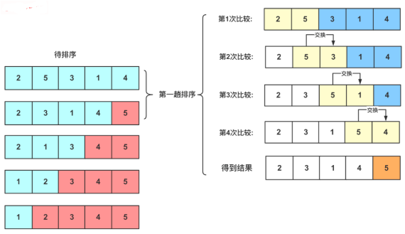
基本上Bubble Sort只在学习时有点意义,实际编程和项目中,没有人会使用这个算法,它太慢了...
参考实现(C语言):
void bubble(int a[], size_t n){
    if (n > 1) {
        size_t i,j;

        for (i=0; i<n-1; ++i) {
            for (j=0; j<n-i-1; ++j) {
                if (a[j] > a[j+1])
                    swap(a+j, a+j+1);
            }
        }
    }
}
比较临近两个元素,一步步将最大或最小的那个推上去,就像泡泡一样,缓慢从水底升起。第1个泡是最大或最小的,第2个泡是次大或次小的。比较的次数只与input size有关,swap的次数与array中元素的初始顺序有关。当输入的array有序时,swap次数为0,当输入的array倒序时,比较的次数与swap的次数相同,均为最大值。
比Bubble Sort好一点点,只是减少了不必要的swap动作。
参考实现(C语言):
void selects(int a[], size_t n){  // conflict name with select
    size_t i,j,k;

    for (i=n; i>1; --i) {
        k = 0;
        for (j=1; j<i; ++j)
            if (a[k] <= a[j]) // = gives stable
                k = j;
        if (k != j-1)
            swap(a+k, a+j-1);
    }
}
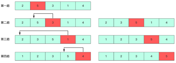
在每一个内循环中,找出(选择)最大的那个,用k定位,最后如果k的位置不对,执行swap。选择排序比冒泡排序快一些,因为在每一轮迭代中,它会比较N次,但最多只交换1次。这种快,在于Hidden Constant这个层面,select sort has smaller hidden constant。But select sort and bubble sort have the same asymptotic upper bound!在实践中,hidden constant带来的性能优势,有时也是非常可观的!
其实,Heapsort就是选择排序!只是Heapsort采用了一种巧妙的方法来实现最大或最小item的选择,但其思想内核,就是选择排序!
Select sort每个迭代选择一个element出来,放在恰当的位置上。Insert sort每个迭代给element选择一个合适的插入位置。
参考实现(C语言):
/* If data is linked in memory by pointer, by using insert algorithm,
 * there is no need to move elements. We could directly modify the
 * pointers to complete the insert action. That would be more efficient.
 * Below is an implementation of the idea of insert on int array. */
void insert(int a[], size_t n){ // stable
    int t;
    size_t i,j;

    for (i=1; i<n; ++i) {
        t = a[i];
        for (j=i; j>0&&a[j-1]>t; --j);
        memmove(a+j+1, a+j, sizeof(int)*(i-j));  // cannot be memcpy
        a[j] = t;
    }
}
void insert2(int a[], size_t n){ // stable
    int t;
    size_t i,j;

    for (i=1; i<n; ++i) {
        t = a[i];
        for (j=i; j>0; --j)
            if (a[j-1] > t)
                a[j] = a[j-1];
            else
                break;
        a[j] = t;
    }
}
从在
int array上的测试结果来看,性能排序为:Insert > Selects > Bubble。Insert比Selects快一点点,但比Bubble快了一个数量级。上面的参考实现,insert2最快!
插入排序算法的关键在于,在已经有序的数据区中寻找插入的位置。二分查找插入排序算法结合查找算法,使用二分查找的方式来寻找插入位置,比单纯的循环遍历查找更快!下面是参考实现:
/* binary insert */
void binsert(int a[], size_t n){
    int t;
    size_t i,j,low,mid,high;

    for (i=1; i<n; ++i) {
        t = a[i];
        /* binary search */
        low = 0;
        high = i-1;
        while (low < high) {
            mid = (low+high) / 2;
            if (a[mid] > t) high = mid;
            else low = mid + 1;
        }
        /* here we get low == high */
        if (a[low] > t) j = low;
        if (a[low] <= t) j = low + 1;
        if (j == i) continue;
        memmove(a+j+1, a+j, sizeof(int)*(i-j));
        a[j] = t;
    }
}
void binsert2(int a[], size_t n){
    int t;
    size_t i,j,k,low,mid,high;

    for (i=1; i<n; ++i) {
        t = a[i];
        /* binary search */
        low = 0;
        high = i-1;
        while (low < high) {
            mid = (low+high) / 2;
            if (a[mid] > t) high = mid;
            else low = mid + 1;
        }
        /* here we get low == high */
        if (a[low] > t) j = low;
        if (a[low] <= t) j = low + 1;
        if (j == i) continue;
        k = i;
        while (k != j) {
            a[k] = a[k-1];
            k--;
        }
        a[j] = t;
    }
}
结合Binary Search的Insert Sort,并没有改变时间复杂度,它变得更快,同样也是因为那个Hidden Constant更小的缘故!
二叉树排序,就是insertion sort,只是插入的动作变成了插入BSTree而已,内核思想是一样的。
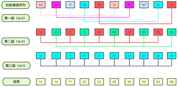
希尔排序是非稳定的排序算法,因DL.Shell于1959年提出而得名。希尔排序可以理解为跳跃版的插入排序。
从此算法的实现上看,有好多for loop的嵌套,但它的速度真的非常快!不能单纯地用for loop嵌套数量来断言算法的时间复杂度,这样简单粗暴得出的结论有时不够tight,很多快速的算法,实现都很复杂。
插入排序在数据量很大,或者数据的移动太多时,会导致效率低下。很多排序算法都会想办法对数据进行分而治之,希尔排序就是以一种特殊的方式对数据进行预处理,考虑到了「数据量和有序性」两个方面纬度来设计算法。使得序列前后之间小的尽量在前面,大的尽量在后面,进行若干次的分组计算交换后,最后一遍计算,即是一趟经典的插入排序。
希尔排序需要选一组递减的整数作为增量序列,不同的增量序列,算法性能也有所不同。下面的参考实现,遵循原始的shell排序算法,其增量序列为不断地除2,直到最后的1。希尔排序的优化主要是针对增量序列的优化,有Hibbard增量序列、Knuth增量序列、Sedgewick增量序列等等,这部分本文不做展开。
参考实现(C语言):
void shell(int a[], size_t n){
    int t;
    size_t i,j,k,u;

    for (i=n/2; i>0; i/=2) {          // define distance
        for (j=0; j<i; ++j) {         // rounds of insert
            for (k=i+j; k<n; k+=i) {  // single insert
                t = a[k];
                for (u=k; u>=i; u-=i) {
                    if (a[u-i] > t)
                        a[u] = a[u-i];
                    else
                        break;
                }
                a[u] = t;
            }
        }
    }
}
Shell排序的最后一次迭代,就是一次标准的insert排序。对于insert排序来说,数据越有序,其性能越高,当输入数据完全有序的时候,insert排序的时间复杂度为\(O(N)\),这是Best Case情况下的时间复杂度。
void shell2(int a[], size_t n){
    int t;
    size_t i,j,k,u;

    for (i=n/2; i>0; i/=2) {          // define distance
        if (i == 1)
            binsert(a, n);
        else {
            for (j=0; j<i; ++j) {         // rounds of insert
                for (k=i+j; k<n; k+=i) {  // single insert
                    t = a[k];
                    for (u=k; u>=i; u-=i) {
                        if (a[u-i] > t)
                            a[u] = a[u-i];
                        else break;
                    }
                    a[u] = t;
                }
            }
        }
    }
}
希尔排序是将待排序的数组元素按位置下标的一定增量分组,逻辑上分成多个子序列,然后对各个子序列进行直接插入排序算法排序。算法最外层循环逐渐缩减增量,直到增量为1时,进行最后一次直接插入排序,排序结束。
希尔排序是基于插入排序的以下两点性质而提出的改进算法:
递归算法的空间复杂度,需要额外考虑递归深度,递归越深,需要的调用栈空间就越大。递归版本的merge sort,递归深度仅为\(\log{n}\),单独分析递归部分,需要的空间为\(c\log{n}\),这属于很好的情况。由于merge sort算法还需要\(\Theta(n)\)的辅助空间,递归部分的空间,因为是个small term,就被省略掉了。
下面是自下而上的非递归参考实现,我比较喜欢这个实现,代码量小:
int merge(int a[], size_t n){
    if (n > 1) {
        size_t i,j,k,s,hs,p;
        int *t = (int*)malloc(sizeof(int)*n);
        if (!t)
            return 1;

        for (s=2; s<n*2; s*=2) {
            hs = s/2;
            p = 0;
            for (i=0; i<n; i+=s) {
                j = i;
                k = i + hs;
                while (p<i+s && p<n) {
                    if (j==i+hs && k<i+s) {
                        t[p++] = a[k++]; continue;
                    }
                    if (k==i+s && j<i+hs) {
                        t[p++] = a[j++]; continue;
                    }
                    if (k>=n && j<n) {
                        t[p++] = a[j++]; continue;
                    }
                    t[p++] = a[j]<a[k]?a[j++]:a[k++];
                }
            }
            memcpy(a, t, sizeof(int)*n);
        }
        free(t);
    }
    return 0;
}
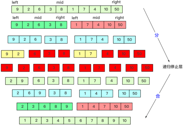
这个图很赞:
下面是自上而下的递归版本:
void _merge(int a[], int *t, size_t li, size_t m, size_t ri){
    size_t i = li;
    size_t j = m+1;
    size_t k = 0;
    size_t len = ri - li + 1;

    while (k < len) {
        if (i == m+1) {
            t[k++] = a[j++]; continue;
        }
        if (j == ri+1) {
            t[k++] = a[i++]; continue;
        }
        t[k++] = a[i]<a[j]?a[i++]:a[j++];
    }
    memcpy(a+li, t, sizeof(int)*len);
}

void _merge_r(int a[], int *t, size_t li, size_t ri){
    if (li < ri) {
        size_t m = (li+ri)/2;
        _merge_r(a, t, li, m);
        _merge_r(a, t, m+1, ri);
        _merge(a, t, li, m, ri);
    }
}

/* merge sort, recursive version */
int merge_r(int a[], size_t li, size_t ri){
    if (li < ri) {
        int *t = (int*)malloc(sizeof(int)*(ri-li+1));
        if (!t)
            return 1;
        _merge_r(a, t, li, ri);
        free(t);
    }
    return 0;
}
算法逻辑示意图:
从测试结果看,merge_r递归版本总是要比merge非递归版本快一丢丢!
相对于merge sort而言,heapsort没有递归,无需额外空间,时间复杂度与merge sort一样,均为理论上最优的asymptotic upper bound!但heapsort有一个缺点:不稳定。
堆是一棵完全二叉树(complete binary tree),分为大根堆和小根堆,完全二叉树中所有节点均大于等于(或小于等于)它的孩子节点,所以这里就分为两种情况:
max heap。min heap。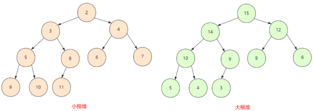
A complete binary tree is a binary tree in which every level, except possibly the last, is completely filled, and all nodes in the last level are as far left as possible.
完全二叉树采用数组而不是链表存储,从node到其children nodes,计算index就可以了。按照惯例,index从0开始,假设某node在array中的index是k,那么,它的两个子节点的index分别是2k+1和2k+2。
下面是Heapsort的C代码参考实现:
/* The Complete Binary Tree has a very import feature:
 * if i is index+1, which means index starts from one, not zero,
 * a[2i] is the left node of a[i], a[2i+1] is just the right node,
 * so, a[i/2] is always the parent of a[i],
 * so, if there are n nodes, a[n/2] is the last node which has leaves. */

/* Adjust heap, assuming from a[s+1] to a[e] is already an adjusted heap.
 * We only need to find the right place for a[s]. */
static void
_heap_adjust(int a[], size_t s, size_t e)  // s and e are index+1
{
    size_t i;

    for (i=s*2; i<=e; i*=2) {
        if (i+1<=e && a[i-1]<a[i]) ++i;  // find the bigger child
        if (a[s-1] < a[i-1]) {
            swap(a+s-1, a+i-1);
            s = i;
        }
        else break;
    }
}

void heapify(int a[], size_t n){
    if (n > 1) {
        size_t i;

        /* create big heap  */
        for (i=n/2; i>0; --i) {
            _heap_adjust(a, i, n);
        }

        /* sorting */
        for (i=n; i>1; --i) {
            swap(a, a+i-1);
            _heap_adjust(a, 1, i-1);
        }
    }
}
以上代码,在数组的基础上,先调整heap,调整完后,最大的数就在顶点,然后将最大的数放交换到最后,继续调整缩小后的heap,继续交换......
快速排序(Quicksort)结合了分治的思想,由C.A.R. Hoare在1962年提出。快速排序的基本思想是:挖坑填数 + 分治法。
快排需要将序列变成两个部分,左序列全部小于一个数,右序列全部大于一个数,这样就完成了Divide。然后利用递归的方法,将左序列当成一个完整的序列再进行排序,同样把右序列也当成一个完整的序列进行排序。其中这个用来区分左右序列的数,在这个序列中是可以随机选取的,或取最左边,或取最右边,当然也可以随机位置。但通常情况,我们取最左边的那个数。
参考实现(C语言):
void quick(int a[], size_t li, size_t ri){
    if (li >= ri) return;
    size_t i,p;

    p = li;
    for (i=li+1; i<=ri; ++i) {
        if (a[li] > a[i])
            if (++p != i)
                swap(a+p, a+i);
    }
    swap(a+li, a+p);

    quick(a, li, p);  // p-1 may cause overflow.
    quick(a, p+1, ri);
}
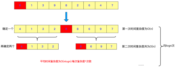
快排的worst case为,输入序列已经有序,而算法每次都选最右边或最左边的数作为pivot,此时就是\(O(n^2)\)的时间复杂度。为了避免出现这样crazy bad的情况,可以对pivot的选择进行随机化处理,即随机选择一个数作为pivot。这样的算法叫做Randomized Algorithm,此时期望的时间复杂度为\(O(n\log{n})\)。实践中,快排的速度是很快的,很多实现都采用randomized pivot的方法。
证明Qsort的Expected Running Time
构建BSTree,然后inorder遍历。
空间复杂度相对较大,BSTree的每个节点,都需要空间。下面是一个C语言的参考实现:
typedef struct bstree_node {
    int val;
    size_t count;
    struct bstree_node *left;
    struct bstree_node *right;
} BSTNODE;


static BSTNODE* insert_bstree(BSTNODE *root, int a, BSTNODE *node){
    if (root == NULL) {
        node->left = node->right = NULL;
        node->val = a;
        node->count = 1;
        root = node;
    }
    else if (a < root->val) {
        root->left = insert_bstree(root->left, a, node);
    }
    else if (a == root->val) {
        root->count++;
    }
    else if (a > root->val) {
        root->right = insert_bstree(root->right, a, node);
    }
    return root;
}


static void walk_bstree(int a[], BSTNODE *root, size_t *i){
    if (root != NULL) {
        walk_bstree(a, root->left, i);
        while (root->count--)
            a[(*i)++] = root->val;
        walk_bstree(a, root->right, i);
    }
}


int bstree(int a[], size_t n){
    if (n > 1) {
        BSTNODE *bmem = (BSTNODE*)malloc(sizeof(BSTNODE)*n);
        if (bmem == NULL) return 1;
        size_t *mi = (size_t*)malloc(sizeof(size_t));
        if (mi == NULL) {
            free(bmem);
            return 1;
        }
        BSTNODE *root = NULL;

        for (size_t i=0; i<n; ++i)
            root = insert_bstree(root, a[i], bmem+i);

        *mi = 0;
        walk_bstree(a, root, mi);
        free(bmem);
    }
    return 0;
}
既要得到遍历的顺序性,还要快速查找,可考虑使用BSTree结构。但现在都不会直接使用原始的BSTree,而是使用它的各种自带平衡属性的变体,比较著名的就是Red-Black-Tree。
从count sort开始,学习研究non-comparison排序算法,这类排序算法对输入数据有些特殊要求,应用范围有限制。
计数排序,就是计数,counting每个key出现的次数,通过counting的值,直接就能得到排序后每个key对应数据的位置。此算法适合key值跨度不大,并且没有负数的场景。
下面是一个用Python写的算法原理说明版(对比pseudocode,我更喜欢写Python):
def count_sort(lst: list[int]) -> list[int]:
    """ count sort (https://cs.pynote.net) """
    size = len(lst)
    # non-negative element
    for i in range(size):
        assert lst[i] >= 0
    # value range
    value_size = max(lst) + 1
    # count
    count = [0] * value_size
    for i in range(size):
        count[lst[i]] += 1
    for i in range(1,value_size):
        count[i] += count[i-1]
    # result start from index 1
    result = [0] * (size+1)
    for i in reversed(range(size)):
        result[count[lst[i]]] = lst[i]
        count[lst[i]] -= 1
    return result[1:]


# test
a = [4,2,0,0,3,1,5,3,7,1,8]
b = count_sort(a)
assert b == sorted(a)
a = [2,5,4,2,3,1,5,3,7,6,7,1,8,0,0,1,0,0,9,9,2,9,9]
b = count_sort(a)
assert b == sorted(a)
下面是本文最后测试的C语言版本:
int get_max(int a[], size_t n){
    assert(n != 0);
    int t = a[0];
    for (size_t i=1; i<n; ++i)
        if (t < a[i]) t = a[i];
    return t;
}

int get_min(int a[], size_t n){
    assert(n != 0);
    int t = a[0];
    for (size_t i=1; i<n; ++i)
        if (t > a[i]) t = a[i];
    return t;
}

int count(int a[], size_t n, size_t mem_limit){
    if (n > 1) {
        if (mem_limit == 0) return 3;
        size_t i,j=0;
        int m = get_min(a, n);
        int k = get_max(a, n);
        size_t mlen = k-m+1;
        if (mlen == 0) {  // int overflow
            if (sizeof(size_t) > sizeof(int))
                mlen = ((size_t)max_int()+1)*2;  // int size
            else if (sizeof(size_t) == sizeof(int))
                mlen = -1;  // biggest size_t
            else assert(0);
        }
        /* memory limit check  */
        if (mlen > mem_limit) return 3;
        /* start malloc */
        UINT8 *counter = (UINT8*)malloc(mlen);
        if (counter == NULL) return 1;  // OOM
        memset(counter, 0, mlen);
        /* count */
        for (i=0; i<n; ++i) {
            if (counter[a[i]-m] == 255) {
                free(counter);
                return 2;  // too man duplicated
            }
            counter[a[i]-m]++;
        }
        /* sort */
        for (i=0; i<mlen; ++i)
            while (counter[i]--) a[j++] = i + m;
        free(counter);
    }
    return 0;
}
支持长度不一致的数字。将Count排序应用在对单个数字进行排序上,就规避了其可能需要很大内存的问题。个人认为这个算法不管有没有用处,还是很精妙的...
def _digit(n, curr):
    s = str(n)
    l = len(s)
    if curr > l:
        return 0
    return int(s[l-curr])


def single_digit_count_sort(lst: list[int], curr) -> list[int]:
    """ single digit count sort (https://cs.pynote.net) """
    assert curr > 0
    count = [0] * 10
    for n in lst:
        d = _digit(n, curr)
        count[d] += 1
    for i in range(1,10):
        count[i] += count[i-1]
    r = [0] * (len(lst)+1)
    for n in reversed(lst):
        d = _digit(n, curr)
        r[count[d]] = n
        count[d] -= 1
    return r[1:]


def count_msd(lst, lo, hi, curr):
    """ most significant digit count sort (https://cs.pynote.net) """
    if curr==0 or hi-lo<2:
        return
    lst[lo:hi] = single_digit_count_sort(lst[lo:hi], curr)
    digit = 10  # not a valid single digit
    for i,n in enumerate(lst[lo:hi],lo):
        s = str(n)
        l = len(s)
        if l < curr:
            continue
        d = int(s[l-curr])
        if d != digit:
            count_msd(lst, lo, i, curr-1)
            digit = d
            lo = i
    # last range
    count_msd(lst, lo, i+1, curr-1)  # i would not be +1 when end loop


a = [135,34,0,232,2123,7]
print(single_digit_count_sort(a,4))
print(single_digit_count_sort(a,3))
print(single_digit_count_sort(a,2))
print(single_digit_count_sort(a,1))
count_msd(a, 0, 6, 4)
print(a)
a = [413, 15, 8, 35, 259, 38, 7, 913, 818, 9]
count_msd(a, 0, 10, 3)
print(a)

import random
for _ in range(100):
    a = [random.randint(0,9999) for _ in range(1000)]
    b = a[:]
    count_msd(a, 0, 1000, 4)
    assert a == sorted(b)
如果是对纯数字进行排序,真的可以实现线速!
Radix sorting常用于需要对多个field进行排序的场景。比如时间份年月日,先对日期排序,再对月份排序,最后对年份排序,最后得到的就是一个有序的数据。在对每个field排序时,看《CLRS》上说,一般常常选择count sort算法配合(对单个数字进行count排序)。CS430教授的课堂上,使用了一种看起来像是bucket排序的方法(其实是FIFO的Queue),这种方法更好,可以有效减少数据copy的次数。
假设对一组数字进行Radix排序,一定要从个位开始,十位,百位....即从低位开始...
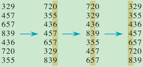
下面是Python版Radix排序参考实现,仅用来示意算法逻辑,代码如下:
def radix_sort(lst: list[int]) -> list[int]:
    """ radix sort (https://cs.pynote.net) """
    width = len(str(lst[0]))
    # same width
    for i in lst:
        assert width == len(str(i))
    # radix sort
    a = lst[:]
    for i in reversed(range(width)):
        fifo = [[] for i in range(10)]
        for n in a:
            fifo[int(str(n)[i])].append(n)
        a = []
        for f in fifo:
            a += f
        # print(a)
    return a


a = [4,2,0,0,3,1,5,3,7,1,8]
b = radix_sort(a)
assert b == sorted(a)
a = [254,231,537,671,800,100,992,916]
b = radix_sort(a)
assert b == sorted(a)
a = ['2154','2731','5337','6571','8900','1400','9292','9616']
b = radix_sort(a)
assert b == sorted(a)
时间复杂度\(O(dn)\),d表示field数量,比如数字的位数,n表示待排序元素的数量。
下面是用于本文后面测试的C语言参考实现:
/* Both radix and count are based on bucket sort idea!  */
typedef struct intdata {
    int val;
    struct intdata *link;  // to next
} INTD;

typedef struct {
    UINT radix;
    INTD *head;
    INTD *tail;
} RADIX;

/* radix is just like base */
UINT get_radix(int a, UINT order){
    a = abs(a);
    for (UINT i=0; i<order; ++i) a /= 10;
    return a%10;
}

/* pos: boundary between negative and positive int,
 * pos is the first positive int position. */
size_t split_np(int a[], size_t n) {
    size_t pos=0,i;

    while (a[pos]<0 && pos<n) ++pos;
    if (pos != n) {
        for (i=pos+1; i<n; ++i)
            if (a[i] < 0) {
                swap(a+i, a+pos++);
            }
    }
    return pos;
}

static int
distribute(int a[], RADIX radix[], INTD *ad, size_t si, size_t n, UINT order)
{
    size_t i,j,k=0;
    INTD *t;

    for (i=si; i<n; ++i) {
        j = get_radix(a[i], order);
        if (j != 0) k=1;
        t = ad + i - si;
        t->val = a[i];
        t->link = NULL;
        if (radix[j].head == NULL) {
            radix[j].head = t;
            radix[j].tail = t;
        }
        else {
            radix[j].tail->link = t;
            radix[j].tail = t;
        }
    }
    return k;
}

static void
collect(int a[], RADIX radix[], size_t si, int ascend)
{
    size_t i,j=si;
    INTD *t;
    UINT b[] = {0,1,2,3,4,5,6,7,8,9};

    if (ascend == 0)
        for (i=0; i<10; ++i) b[i] = 9-i;

    for (i=0; i<10; ++i) {
        while (radix[b[i]].head != NULL) {
            t = radix[b[i]].head;
            radix[b[i]].head = radix[b[i]].head->link;
            a[j++] = t->val;
        }
    }
}

int radix(int a[], size_t n){
    if (n > 1) {
        UINT k,order;
        RADIX radix[] = {
                    {0, NULL, NULL},
                    {1, NULL, NULL},
                    {2, NULL, NULL},
                    {3, NULL, NULL},
                    {4, NULL, NULL},
                    {5, NULL, NULL},
                    {6, NULL, NULL},
                    {7, NULL, NULL},
                    {8, NULL, NULL},
                    {9, NULL, NULL},
              };
        /* first of all, try to get enough memory */
        INTD *ad = (INTD*)malloc(sizeof(INTD)*n);
        if (ad == NULL) return 1;

        const size_t pos = split_np(a, n);
        /* negative part */
        if (pos != 0) {
            order = 0;
            do {
                k = distribute(a, radix, ad, 0, pos, order++);
                collect(a, radix, 0, 0);
            } while (k);
        }

        /* positive part */
        if (pos != n) {
            order = 0;
            do {
                k = distribute(a, radix, ad, pos, n, order++);
                collect(a, radix, pos, 1);
            } while (k);
        }

        free(ad);
    }
    return 0;
}
假设输入是数字,数字的每个位都被处理之后,就可以提前将其输出了。参考实现如下,用了两个list of queue来回倒:
from collections import deque


def radix_sort_2(lst: list[int]) -> list[int]:
    """ radix sort,
    support non-same-length number (https://cs.pynote.net) """
    r = []
    mfifo = [deque() for _ in range(9)]
    mfifo.append(deque((n,str(n),len(str(n))) for n in lst))
    afifo = [deque() for _ in range(10)]
    cur = 0
    while len(r) < len(lst):
        for dq in mfifo:
            while dq:
                t = dq.popleft()
                if t[2] == cur:
                    r.append(t[0])
                    continue
                afifo[int(t[1][t[2]-cur-1])].append(t)
        mfifo, afifo = afifo, mfifo
        cur += 1
    return r


a = [3,22,123,69876,50,422,3333,21,1]
print(radix_sort_2(a))

import random
for _ in range(100):
    a = [random.randint(0,999999) for _ in range(100)]
    b = radix_sort_2(a)
    assert b == sorted(a)
时间复杂度为\(O(n+k)\),n是输入数字的个数,k是所有数字位数的总和。这个版本的mfifo和afifo相互倒数据,可以减少数据copy的次数,感觉是radix排序的一个更优的实现版本!
Buckets之间有序,保持每个Bucket内有序,最后一把收。
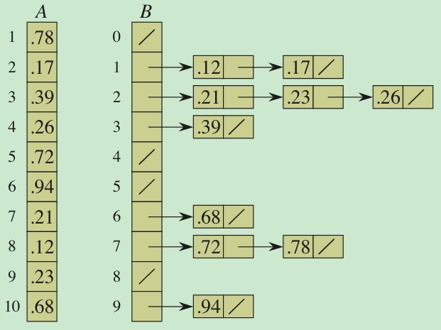
Bucket排序对input有个假设,即input数据是均匀分布的。这很好理解,input数据需要均匀的放入每个bucket之中。如果所有input数据都放入了一个bucket,就变成insert排序了。与Radix排序中所用到的FIFO不同,进入同一个Bucket内的元素,在Bucket内部要保持顺序,而且进出仅一次就完成排序。Radix排序需要反反复复进出好几次FIFO。
这几个non-comparison sorting algorithm的差异有些微妙...需好好体会...
这部分测试是很早以前做的,也许不够严谨和规范,不想改了,所有数据进作为参考,C语言的实现代码本文都已经提供。测试代码在这里(private):https://github.com/xinlin-z/internal_sorting_algorithm
$ python3 utest.py -v

# common.c:
sizeof(int) =  4
sizeof(size_t) =  8

test_cmp_int (__main__.test_common_c) ... ok
test_max_int (__main__.test_common_c) ... ok
test_min_int (__main__.test_common_c) ... ok

# sort.c:
sizeof(int) =  4
sizeof(size_t) =  8

test_binsert (__main__.test_sort_c) ... ok
test_binsert2 (__main__.test_sort_c) ... ok
test_btree (__main__.test_sort_c) ... ok
test_bubble (__main__.test_sort_c) ... ok
test_count (__main__.test_sort_c) ... ok
test_get_max (__main__.test_sort_c) ... ok
test_get_min (__main__.test_sort_c) ... ok
test_get_radix (__main__.test_sort_c) ... ok
test_heapify (__main__.test_sort_c) ... ok
test_insert (__main__.test_sort_c) ... ok
test_insert2 (__main__.test_sort_c) ... ok
test_merge (__main__.test_sort_c) ... ok
test_merge_r (__main__.test_sort_c) ... ok
test_quick (__main__.test_sort_c) ... ok
test_radix (__main__.test_sort_c) ... ok
test_selects (__main__.test_sort_c) ... ok
test_shell (__main__.test_sort_c) ... ok
test_shell2 (__main__.test_sort_c) ... ok
test_split_np (__main__.test_sort_c) ... ok

----------------------------------------------------------------------
Ran 22 tests in 12.844s

OK
$ python3 test_sort_time.py
# test sort time (cpu) with same data:

sizeof(int) = 4
sizeof(size_t) = 8
Data1: 200000 integers in random from -500 to 500 (many duplicated)
     Algo Name                   Time(s)
1    count                    0.0002865390
2    radix                    0.0063802410
3    btree                    0.0100811730
4    merge_r                  0.0127625810
5    merge                    0.0130818440
6    quick                    0.0144666640
7    heapify                  0.0145566040
8    shell                    0.0149387610
9    np.sort(numpy)           0.0159584780
10   qsort(glibc)             0.0162465800
11   shell2                   0.0187523920
12   list.sort(python)        0.0216216080
13   sorted(python)           0.0228952610
14   binsert2                 0.6138220350
15   binsert                  0.6154471680
16   insert2                  3.3854721020
17   insert                   4.6864306390
18   selects                  7.7486197970
19   bubble                   48.3289254720

Data2: 200000 integers in random from -2147483648 to 2147483647
     Algo Name                   Time(s)
1    quick                    0.0121813170
2    merge_r                  0.0154146260
3    merge                    0.0159740240
4    heapify                  0.0164701320
5    shell                    0.0185461380
6    qsort(glibc)             0.0195465400
7    radix                    0.0201735410
8    np.sort(numpy)           0.0210044280
9    shell2                   0.0234900200
10   btree                    0.0437949200
11   sorted(python)           0.0453653430
12   list.sort(python)        0.0466786440
13   binsert                  0.5995638920
14   binsert2                 0.6202496610
15   insert2                  3.3880157650
16   insert                   4.6766841610
17   selects                  7.7102677510
18   bubble                   48.3651019260
19   count                    E:3
本文链接:https://cs.pynote.net/ag/202206101/
-- EOF --
-- MORE --