统计和概率

Last Updated: 2024-03-14 12:45:32 Thursday

-- TOC --

Basic Concepts
Numerical Measures
Bivariate Data
Probability
Discrete Distributions
The Normal Probability Distribution
- Continuous Random Variable
Normal Probability Distribution
Sampling Distribution
Large-Sample Estimation

统计是数学应用的一个分支，与我们的日常生活以及计算机算法有很多联系，很需要Common Sense和Logical Thinking。初学统计，不需要深入到对计算公式的证明，只需要理解和应用。

Basic Concepts

Population表示全体，通常统计手段是难以覆盖整个population的，因此需要一个Sample，we try to describe or predict the behavior of the population on the basis of information obtained from a representative sample from that population.
Descriptive statistics consists of procedures used to summarize and describe the important characteristics of a set of measurements.
Inferential statistics consists of procedures used to make inferences about population characteristics from information contained in a sample drawn from this population.
An experimental unit is the individual or object on which a variable is measured, and the data value is called a single measurement.
Variable，变量的类型：quanlitative（描述性质的，分类用的）和quantitative（描述数量的），quantitative有分为discrete（离散量）和continuous（连续量）。
frequency，频率，（某种单位下的）次数或数量，可解释为 number of measurements。
relative frequency，$\cfrac{frequency}{n}$，n是样本总数。
percent，$100\times \text{relative frequency}$

Quanlitative的量类似于分类，图形化表示常用柱状图bar chart或饼图pie chart。而Quantitative的量，常常用直方图Histogram来表现数据的分布（data distribution）。

Bar Chart与Histogram的区别

bar chart用于quanlitative数据，每个类别一个bar，bar与bar之间有间隔分割。
historgram用于quantitative数量，也有bar，但bar与bar之间紧挨着，bar的宽度和数量人为设定，采用left inclusion method。

Remember, though, that different samples from the same population will produce different histograms, even if you use the same class boundaries. However, you can expect that the sample and population histograms will be similar. As you add more and more data to the sample, the two histograms become more and more alike. If you enlarge the sample to include the entire population, the two histograms will be identical!

除了用图形来表达和展示数据（数据可视化），还可以用一些量化的方法，来表达数据的某些性质。These measures are called parameters when associated with the population, and they are called statistics when calculated from sample measurements.

Measures of Center

描述一组数据的中心性质。

算数平均数Mean

sample mean： $\bar x=\cfrac{\sum x_i}{n}$
population mean： $\mu$

关于各种平均数的总结

中位数Median

将一组数据进行排序后，位置在中间的那个数，或者中间的两个数的算数平均值。比如LeetCode的第4题，两有序数组的中间值。

Median is less sensitive to extreme values or outliers! If a distribution is strongly skewed by one or more extreme values, you should use the median rather than the mean as a measure of center.

Median对outliers不敏感，而Mean非常敏感。

Mode

The mode is the category that occurs most frequently, or the most frequently occurring value of x. When measurements on a continuous variable have been grouped as frequency or relative frequency histogram, the class with the highest peak or frequency is called the modal class, and the midpoint of that class is taken to be the mode. It is possible for a distribution of measurements to have more than one mode.

学点英语：Think of modal as relating to some "mode" or form. The English word modal has long been used as a term in logic and statistics, such as "modal values". 一般情况下，每个modal value都对应了一个distribution，distribution可以理解为mode或form。

用Numpy计算mean和median

>>> np.mean((1,2,3,3))
2.25
>>> np.median((1,2,3,3))
2.5

Measures of Variability

范围Range

The range, R, of a set of n measurements is definied as the difference between the largest and smallest measurements.

离差Deviation

$x_i - \bar{x}$，有正有负

差方Variance

variance of population: $\sigma^2=\cfrac{\sum(x_i-\mu)^2}{N}$
variance of sample: $s^2=\cfrac{\sum(x_i-\bar{x})^2}{n-1}=\cfrac{\sum{x_i^2}-\cfrac{(\sum{x_i})^2}{n}}{n-1}$

为什么分母是n-1？：简单理解，就是当分母是n-1时，能更好的估算population的差方值，比使用n更好。（只是更好！原因不详...?）

标准差Standard Diviation

$s=\sqrt{s^2}$，正值

The value of s is always greater than or equal to zero.
The larger the value of $s^2$ or s, the greater the variability of the data set.
If $s^2$ or s is equal to zero, all the measurements must have the same value.
In order to measure the variability in the same units as the original observations, we compute the s. 标准差的单位与sample单位一致。

用Numpy计算var和std

默认ddof=0，当ddof=1时，计算var的分母就是n-1。

>>> import numpy as np
>>> x = [np.random.randn() for i in range(100)]
>>> np.var(x, ddof=1)
0.9932329373836302
>>> np.std(x, ddof=1)
0.99661072509964
>>> np.sqrt(np.var(x,ddof=1))
0.99661072509964

Tchebysheff's Theorem

以俄罗斯数学家Tchebysheff命名的定理，可用来描述任意分布的数据，因此它给出的描述非常保守。

Given a number k greater than or equal to 1 and a set of n measurements, at least $1 - \cfrac{1}{k^2}$ of the measurements will lie within k standard deviations of their mean.

这个定义是保守的，它可以用来描述任何分布的数据，sample或population
$k\ge 1$，可以是个小数
$1 - \cfrac{1}{k^2}$计算出来也可能是个小数，实际应用时round to zero取整

k	$1 - \cfrac{1}{k^2}$	Interval
1	0	$\bar{x}\pm s$
2	$\frac{3}{4}$	$\bar{x}\pm 2s$
3	$\frac{8}{9}$	$\bar{x}\pm 3s$
2.5	0.84	$\bar{x}\pm 2.5\times s$

Empirical Rule

如果数据呈现mound-shaped形状，此时可以应用所谓的Empirical Rule来分析其分布。其实这就是著名的高斯分布，或正态分布，在自然界中几乎无处不在。这里直接给出一点结论：

Interval	Approximate number of measurements
$\bar{x}\pm s$	68%
$\bar{x}\pm 2s$	95%
$\bar{x}\pm 3s$	99.7%

所谓的牛人，就是处于3倍标准差之外的那些人...千分之三！

对比Tchebysheff定理的数据，就可以看出Tchebysheff有多保守，但它给出了很重要的Low Bound！

Range Approximation of s

不管是Tchebysheff，还是Empirical Rule，都能发现一个规律，绝大部分的measurements都集中在以mean为中心的4倍标准差的这个范围内。因此，下面的计算，可以得到标准差s的估计值：

$s\approx\cfrac{R}{4}$

这是Range与标准差s之间的一个大约的关系，这样计算得到的近似s，可以用来与标准计算得到的s进行比较，这两个值不太可能相等，但如果在一个数量级上，可以判断通过标准计算得到的s值是可信的。这个关系式的系数并不固定为4。Measurements的数量越多，Range的范围就越大，系数就需要更小。教科书中有这样一个table：

Number of Measurements	Expected Ratio of Range to s
5	2.5
10	3
25	4

z-scores

$\text{z-score}=\cfrac{x-\bar{x}}{s}$

从计算公式可以看出，z-score表示距离mean有多少个standard deviation，可正可负，分别表示above the mean或below the mean。表达的是relative standing信息。

对于mound-shaped data：

当z-score绝对值大于2时，可以认为 somewhat unlikely
当z-score绝对值大于3时，可以认为 very unlikely

对于某个measurement，如果它的z-score绝对值很大，就可以怀疑这个measurement是否为outlier，或需要去仔细检查sample的各个环节是否有错误。

Percentile

Percentile是一个值，中文翻译为百分位数，一般在对数据量较大的data set分析时才有意义。比如：60% percentile is x，这表示，在所有的measurements中，有60%的数据小于x，另有（1-60%）=40%的数据大于x。median happens to be 50% percentile。

Quartile，将数据等分成4份，每份25%

Lower quartile, first quartile, Q1, 25% percentile
Second quartile is the median, 50% percentile
Upper quartile, third quaritle , Q3, 75% percentile

还记得偶数（n）个measurements时，median如何计算吗？把中间的两个数加起来算平均值。这实际上是在做linear interpolation。我们在计算Q1和Q3的时候也是这样，具体如下：

Q1的位置为0.25(n+1)，如果不是整数，取此位置左右两边的数，linear interpolation
Q3的位置为0.75(n+1)，如果不是整数，取此位置左右两边的数，linear interpolation
median的位置0.5(n+1)

InterQuartile Range (IQR)

$IQR = Q3 - Q1$

这个range，覆盖了一半的数据。

Boxplot

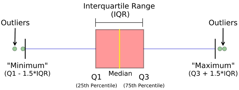
由 min, Q1, median, Q3和max（five-number summary）构成的图形。在Q1和Q3之间画一个box，median的位置画一条线表示。

Lower fence: Q1-1.5IQR
Upper fence: Q3+1.5IQR

不在Lower fence和Upper fence之间的数据，就是outlier，在boxplot中用asterisk(*)表示。排除掉outlier后，再找出min和max，在Q1与min，Q3与max之间，画whiskers。

下面是一个均匀分布数据的boxplot示例：

$boxplot$

Bivariate Data

针对同一个experiment unit，同时有多个不同的measurements，将其中两个放在一起，就形成了bivariate data。比如对每个学生，统计年龄，身高，性别和体重，每个学生统计4个数据，如果将其中两个数据放在一起分析，就形成了bivariate data。

图形化bivariate data，可以并排画bar chart，或者stacked bar chart。如果都是quantitative data，可以画出scatter plot，观察数据间的关系。

Covariance

$s_{xy}=\cfrac{\sum(x_i-\bar{x})(y_i-\bar{y})}{n-1}=\cfrac{\sum{x_iy_i-\frac{(\sum{x_i})(\sum{y_i})}{n}}}{n-1}$

虽然用s，但有xy下标，还是表示这是covariance。

Correlation Coefficient

$r=\cfrac{s_{xy}}{s_x s_y}$

当x=y时，r=1，自己跟自己的correlation coefficient（相关系数）等于1。
r的取值，在[-1,1]之间，越靠近两端，x和y的线性关系就越强，scatterplot中那条隐约可见的直线，要么向上，要么向下。

用NumPy接口计算Correlation Coefficient

>>> a
(1360, 1940, 1750, 1550, 1790, 1750, 2230, 1600, 1450, 1870, 2210, 1480)
>>> b
(278.5, 375.7, 339.5, 329.8, 295.6, 310.3, 460.6, 305.2, 288.6, 365.7, 425.3, 268.8)
>>> np.corrcoef(a,b)
array([[1.        , 0.92410965],
       [0.92410965, 1.        ]])

a与b，b与a，系数值一样。a与a，b与b，都是1。

Regression（Least-Squares Line）

线性回归分析，bivariate data x and y，不管x和y是什么关系，线性分析都可以提供一个最简单的模型。Regression这个名字，就是回退到最简单的Linear关系的意思。用下面的公式可直接计算线性回归线：

$$\begin{cases} b=r\cdot \left(\cfrac{s_y}{s_x}\right)=\cfrac{s_{xy}}{s_x^2} \\ a=\bar{y}-b\bar{x} \end{cases}$$

The least-squares regression line is: $y=a+bx$

前面这一部分，全是对纯数据进行分析的技术，下面开始进入概率~~！！

Probability

识别出Sample Space和Event，建立概率思考模型。

An experiment is the process by which an observation or measurement is obtained.
A simple event is the outcome that is observed on a single repetion of the experiment.
An event is a collection of simple events. (An event is a subset of the sample space)
Two events are mutually exclusive (disjoint) if , when one event occurs, the other cannot, and vice versa. Simple events are mutually exclusive!
The set of all simple events is called the sample space, S.

Venn diagram （维恩图） can be used to visualize sample space and events. Some experiments can be generated in stages, and the sample space can be displayed in a tree diagram.

从频率的角度理解概率：P(A)表示事件A的概率（probability of event A），n为experiment的次数，f为事件A发生的frequency（次数），有公式如下：

$$P(A)=\lim\limits_{n\rightarrow\infty}\cfrac{f}{n}$$

Each simple event's probability must lie between 0 and 1.
The sum of the probabilities for all simple events in S equals 1.
The probability of an event A is equal to the sum of the probabilities of the simple events contained in A. P(A)等于A所包含simple event的概率的和。
The event S is called the certain event.
The event $\empty$ is called the null event.

Event Relations and Probability Rules

三种基本关系

The union of events A and B, denoted by $A\cup B$, is the event that either A or B or both occur.
The intersection of events A and B, denoted by $A\cap B$, is the event that both A and B occur.
The complement of an event A, denoted by $A^c$, is the event that A does not occur.

Addition Rule

$P(A\cup B)=P(A)+P(B)-P(A\cap B)$

When two events A and B are mutually exclusive, then $P(A\cap B)=0$.

Complement Rule

$P(A^c)=1-P(A)$

Multiplication Rule

$P(A\cap B)=P(A)P(B|A)=P(B)P(A|B)$

| can be read as given.

Independent Event

独立事件：

Two events, A and B, are said to be independence if and only if the probability of event B is not influenced or changed by the occurence of event A, or vice versa.

事件B发生的概率，不会因为事件A是否发生而改变，则B与A是相互独立的事件，此时：

$P(A\cap B)=P(A)P(B)$

$P(B|A)=P(B)$

$P(A|B)=P(A)$

如何判断事件A和B是否Independent？

计算上满足上述等式之一，就是independent。

三个相互独立事件

$P(A\cap B\cap C)=P(A)P(B)P(C)$

更多相互独立的事件，也满足这样的式子，典型如Binomial事件。

Mutually Exclusive Events

Mutually exclusive事件相互排斥，是不可能同时发生的事件，因此，mutually exclusive事件一定是dependent事件，当A与B互斥时，有如下关系：

$P(A\cap B)=0$

$P(B|A)=P(A|B)=0$

$P(A\cup B)=P(A) + P(B)$

如果将mutually exclusive events看做二维空间内的不相交的事件，那么independent events就应该是三维空间内的事件，它们只是发生在不同的二维空间。

Conditional Probability

事件概率的Multiplication Rule，就是Conditional Probability，条件概率。当事件A与B不独立，B的发生与否，影响改变A的概率。把公式换一种写法，也许能看出点不一样的含义：

$P(A|B)=\cfrac{P(A\cap B)}{P(B)}, P(B)\neq 0$

如果是单纯的P(A)，即事件A在整个sample space中发生的概率，可以说这是Unconditional Probability，无条件的事件概率。

Law of Total Probability

Give a set of events $S_1, S_2, S_3, ..., S_k$ that are mutually exclusive and exhaustive and an event A, the probability of the event A can be expressed as:

$$P(A)=\sum_{i=1}^kP(S_i)P(A|S_i)=\sum_{i=1}^kP(A\cap S_i)$$

这非常符合直觉！

$P(S_i)$ is also called prior probability.

Bayes' Rule

$P(S_i|A)=\cfrac{P(S_i)P(A|S_i)}{P(A)}=\cfrac{P(A\cap S_i)}{P(A)}$

$P(S_i|A)$ is also called posterior probability.

贝叶斯概率就是条件概率，它所求的是，当某事件发生时，此事件所对应的“某块拼图”的概率。（将样本空间想象成一个拼图，所有的块相互之间mutually exclusive，放在一起exhaustive）

Discrete Random Variables

用一个变量来表示事件，不同事件对应不同的值，离散值。变量出现某个值，就是对应事件的发生，某个值出现的概率，就是对应事件的发生概率。

A variable x is a random variable if the value that it assumes, corresponding to the outcome of an experiment, is a chance or random event. 随机事件，对应随机变量。

The probability distribution for a discrete random variable is a formula, table or graph that gives the possible values of x, and the probability p(x) associated with each value of x.

事件以及概率用大写字母和大P，随机变量及其概率用小写字母和小写p！

Mean（Expected Value）

Let x be a discrete random variable with probability distribution p(x). The mean or expected value of x is give as:

$$\mu=E(x)=\sum x\cdot p(x)$$

离散随机变量的期望值，就是加权平均数。

Variance and Standard deviation

Let x be a discrete random variable with probability distribution p(x) and mean $\mu$. The variance of x is:

$$\sigma^2=E\left((x-\mu)^2\right)=\sum (x-\mu)^2\cdot p(x)$$

Var也是一个加权平均数。

More about Expection and Variance

Linearity of Expectation

The expection of the sum of two random variables is the sum of their expections. 和的期望等于期望的和。

$E(x+y)=E(x)+E(y)$

Proof:

$\begin{aligned} \sum_{i,j}(x_i+y_j)\cdot p(x_i)p(y_j)&=\sum_{i,j}\left(x_ip(x_i)p(y_j)+y_jp(x_i)p(y_j)\right) \\ &=\sum_{i}x_ip(x_i)\cdot\sum_{j}p(y_j)+\sum_{j}y_jp(y_j)\cdot\sum_{i}p(x_i) \\ &=\sum_{i}x_ip(x_i)+\sum_{j}y_jp(y_j) \end{aligned}$

QED

$E(ax)=a\cdot E(x)$

So, $E(x+x)=E(2x)=2E(x)$

When two random variables are independent,

$E(xy)=E(x)\cdot E(y)$

Variance

$Var(x)=E(x^2)+E^2(x)$

$E(x^2)=Var(x)-E^2(x)$

$Var(ax)=a^2Var(x)$

When two random variables are independent,

$Var(x+y)=Var(x)+Var(y)$

Indicator Random Variable

Indicator Random Variable对应了某一个具体的事件，当此事件发生，变量值为1，当此事件没有发生，变量值为0。Indicator random variables provide a convenient method for converting between probabilities and expectations. Given a sample space S and an event A, the indicator random variable $I(A)$ associated with event A is defined as：

$$I(A)=\begin{cases} 1, &\text{ if A occurs} \\ 0, &\text{ if A does not occur} \end{cases}$$

事件发生的概率，就是此事件绑定的Indicator随机变量的期望。Given a sample space S and an event A in the sample space S , let $X_A=I(A)$. Then $E(X_A)=P(A)$.

Discrete Distributions

Binomial Distribution

A Bernoulli trial is an experiment with only two possible outcomes: success, which occurs with probability p, and failure, which occurs with probability q=1-p. It also be called binomial experiment, which has these five characteristics:

The experiment consists of n identical trials.
Each trial results in one of two outcomes. For lack of a better name, the one outcome is called a success, S, and the other a failure, F.
The probability of success on a single trial is equal to p and remains the same from trial to trial. The probability of failure is equal to (1-p)=q.
The trials are independent.
We are interested in x, the number of S observed during the n trials.

当population size很大时，每次trial对p的影响非常小，可以认为每次trial是独立的，p没有变化。而当population size较小时，每次trial无法独立，p的值会显著变化。

Rule of Thumb，n is sample size, N is population size, if n/N >= 0.05, then the resulting experiment is not binomial。（Actually, now it's another distrubtion called hypergeometric probability distribution. See below.）

抛硬币实验，Population是无穷大，因为就是可以一直抛下去，直到天荒地老...

The Binomial Probability Distribution

A binomial experiment consists of n identical trials with probability of success p on each trial. The probability of k successes in n trials is

$P(x=k)=C_n^k p^k q^{n-k}$
$E(x)=np$
$Var(x)=npq$

Geometric Distribution

Geometric Distribution比Binomial Distribution要简单一点，后者关注的是n次实验k次S的概率，而前者仅关注第k次才出现S的概率。How many trials occur before a success?

$P(x=k)=q^{k-1}p$
$E(x)=1/p$
$Var(x)=q/p^2$

Poisson Distribution

The number of occurences of a special event in a given unit time or space. These events occur randomly and independently.

计算泊松分布，需要事先知道特定时间内事件发生的平均次数。

mean: $\mu$，已知条件
$P(x=k)=\cfrac{\mu^k e^{-\mu}}{k!}$
standard deviation: $\sigma=\sqrt{\mu}$

下面是一些可用泊松分布作为概率分析模型的事件：

某段高速公路在一个特定时间周期内发生事故的次数
呼叫中心的客服在一个特定时间周期内接听电话的次数
在一个小剂量中发现细菌的数量（发现一个算一次）
在一个特定时间周期内，客户到达checkout counter的数量

当n很大，u=np很小时（<7），binomial分布可以用poisson分布来近似。

Hypergeometric Distribution

前面在总结二项分布时就提到，当sample size n远远小于population size N时，就可以应用二项分布。泊松分布中，n很大，而u很小时，也可以用泊松分布来近似二项分布。超几何分布，就是当n不能满足远远小于N的时候，采用的概率分布。

A population contains M successes and N-M failures. The probability of exactly k successes in a random sample of size n is:

$P(x=k)=\cfrac{C_M^k C_{N-M}^{n-k}}{C_N^n}$
$\mu=n\left(\frac{M}{N}\right)$
$\sigma^2=n(\frac{M}{N})(\frac{N-M}{N})(\frac{N-n}{N-1})$

超几何分布其实很好理解，就是我们中学时常常玩的，盒子里有N个球，有红球M个，剩下为绿球，要拿出n个，k个红球的概率。

The Normal Probability Distribution

Continuous Random Variable

显然，不是所有的experiment都能产生discrete数据，比如身高，体重，长宽数据等等，这些都是continuous random variable，叫做连续随机变量。通过大量的采集experiment数据，绘制histogram，可以得到连续随机变量近似的概率分布。

Probability distribution or probability density function (pdf), $f(x)$，概率密度函数，其实就是连续随机变量的概率分布。

$P(x=a)=0$ for continuous random variables，连续随机变量有无限多的取值，等于某个具体值时的概率为0，要让概率不为0，需要在概率密度函数f(x)上做两点间的积分，即两点间在f(x)下形成的区域面积，就是具体的概率。
$P(x\ge a)=P(x>a)，P(x\le a)=P(x<a)$
离散随机变量所有取值的概率相加为1，连续随机变量在两个极值间根据密度函数积分的值为1。

Uniform Random Variable

变量的值均匀分布在一个指定间隔中。比如因为rounding产生的误差。

$f(x)=\frac{1}{b-a}, a\le x \le b$
$\mu=\frac{a+b}{2}$
$\sigma^2=\frac{(b-a)^2}{12}$

Exponential Random Variable

例如超市收银台的等待时间。

$f(x)=\lambda e^{-\lambda x}, x\le 0$
$\mu=\frac{1}{\lambda}$
$\sigma^2=\frac{1}{\lambda^2}$

Relative frequency histogram可能会提供变量数据分布的线索，我们应该选择最适合连续随机变量的分布。不过很幸运，很多场景下连续随机变量的分布，都符合正态分布。

Normal Probability Distribution

这个世界，大部分的连续随机变量的概率分布，都是normal distribtuion，我想这也是normal用词的含义。初始化神经网络的权重，一般都采用标准随机正态分布的数据。

$f(x)=\cfrac{1}{\sigma\sqrt{2\pi}}\ e^{-(x-u)^2/(2\sigma^2)}, \sigma\gt 0, x\in R$

$\sigma$决定了f(x)的形态：$\sigma$越小，曲线越高越窄；$\sigma$越大，曲线越低越宽。

Standard Normal Random Variable

$\mu=0$
$\sigma=1$
概率密度函数的图像在x=0处左右对称

将连续随机变量转换成z-score（平移和缩放），就可以得到标准正态分布：

$z=\cfrac{x-\mu}{\sigma}$

$f(z)=\cfrac{1}{\sqrt{2\pi}}\ e^{-z^2/2}$

转换成标准正态分布后，就可以通过查表计算了。前面的几个概率分布，都有表可以查的...

Sampling Distribution

通过采样数据的分析，来推测总体的参数，from statistics to parameters...

Sampling Plan

The way a sample is selected is called the sampling plan or experimental design. Knowing the sampling plan used in a particular situation will often allow you to measure the reliability or goodness of your inference.

Simple Random Sampling

就是随机选！但是需要了解，现实中完美的随机选择，是难以做到的。（所有可用于inference的采样方法，都有随机因素）

Stratified Random Sampling involves selecting a simple random sample from each of a given number of subpopulations, or strata.

Cluster Random Sampling

1-in-k Systematic Random Sampling

还有一些non-random采样的方法。需要注意，non-random样本可以被描述，但不能用于inference！

Sampling Distribution

The sampling distribution of a statistic is the probability distribution of the possible values of the statistic that results when random samples of size n are repeatedly drawn from the population.

通过不断地随机采样，并计算statistics（numerical measurements of samples），这些数值本身的概率分布，即sampling distribution。

Central Limit Theorem (CLT)

在很一般的情况下，通过random samples得到的sums或means等数据，呈现近似的normal distribution。

If random samples of n observations are drawn from a nonnormal population with finit mean $\mu$ and standard deviation $\sigma$, then, when n is large, the sampling distribution of the sample mean $\bar{x}$ is approximately normally distributed, with mean $\mu$ and standard deviation $\cfrac{\sigma}{\sqrt{n}}$ .

sampling distribution is approximately normal。
mean就是population的mean，mean的std可以通过population的parameter计算，n越大，mean的std就越小。
CLT成立的前提是n要足够大，如果population本就是normal的，或者symmetry，n can be just moderate，否则n就要比较大。（书上说至少要大于30，特别skewed，恐怕还要更大，比如p特别小的binomial）

Tip: If x is normal, $\bar{x}$ is normal for any n. If x is not normal, $\bar{x}$ is approximately normal for large n.

Standard Error

The standard deviation $\cfrac{\sigma}{\sqrt{n}}$ is also called the standard error of the estimator (abbreviated SE). Therefore, the SE of $\bar{x}$ is standard error of the mean (abbreviated $SE(\bar{x})$ or SEM).

所谓的estimator，比如通过采样数据得到的$\bar{x}$，要用它来预测$\mu$，因此有estimator这个说法。

Sampling Distribution of Sample Proportion

If a random sample of n observations is selected from a binomial population with parameter p, then the sampling distribution of the sample proportion $\hat{p}=\cfrac{x}{n}$ will have a mean $p$ and a standard deviation $SE(\hat{p})=\sqrt{\cfrac{pq}{n}}$ where $q=1-p$.

When the sample size n is large, the sampling distribution of $\hat{p}$ can be approximated by a normal distribution. The approximation will be adequate if $np>5$ and $nq>5$.

Binomial分布关注在已知p的情况下，n次trial中，x次S的概率。Sample Proportion关注如何近似p值。

Large-Sample Estimation

前面的内容，都是工具箱里的工具，现在开始进入Statistical Inference！

本文链接：https://cs.pynote.net/math/202310071/

-- EOF --

-- MORE --

k	\(1 - \cfrac{1}{k^2}\)	Interval
1	0	\(\bar{x}\pm s\)
2	\(\frac{3}{4}\)	\(\bar{x}\pm 2s\)
3	\(\frac{8}{9}\)	\(\bar{x}\pm 3s\)
2.5	0.84	\(\bar{x}\pm 2.5\times s\)